pdf graphic with the biggest conected component of the m-DAG
hsa_mDAG_biggerDAG.svg
svg graphic with the biggest conected component of the m-DAG
hsa_mDAG_nl.csv
csv file with the node (MBBs) labels of the m-DAG
hsa_mDAG_structure.csv
csv file with all connected components of the m-DAG
hsa_R_adj.csv
csv file with the adjacency matrix of the reaction graph
hsa_R_nl.csv
csv file with the node (reactions) labels of the reaction graph
hsa_RC.graphml
reaction graph GraphML format
hsa_RC.pdf
reaction graph pdf graphic
hsa_RC.svg
reaction graph svg graphic
hsa_summary.txt
text summary file with the number of MBBs, reactions, etc. in the previous graphs
3.2 Pan & core metabolic graphs
Pan and core metabolic graphs for every group were generated. For instance, one can read the pan and core metabolic graphs generated for the group Algae in the directory (Groups/Algae).
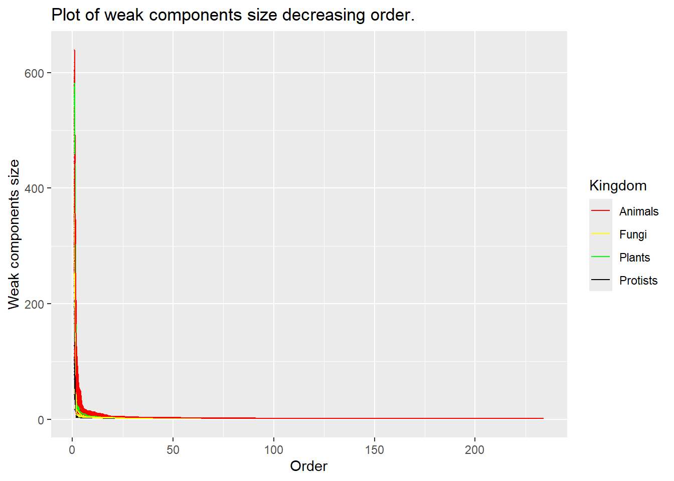
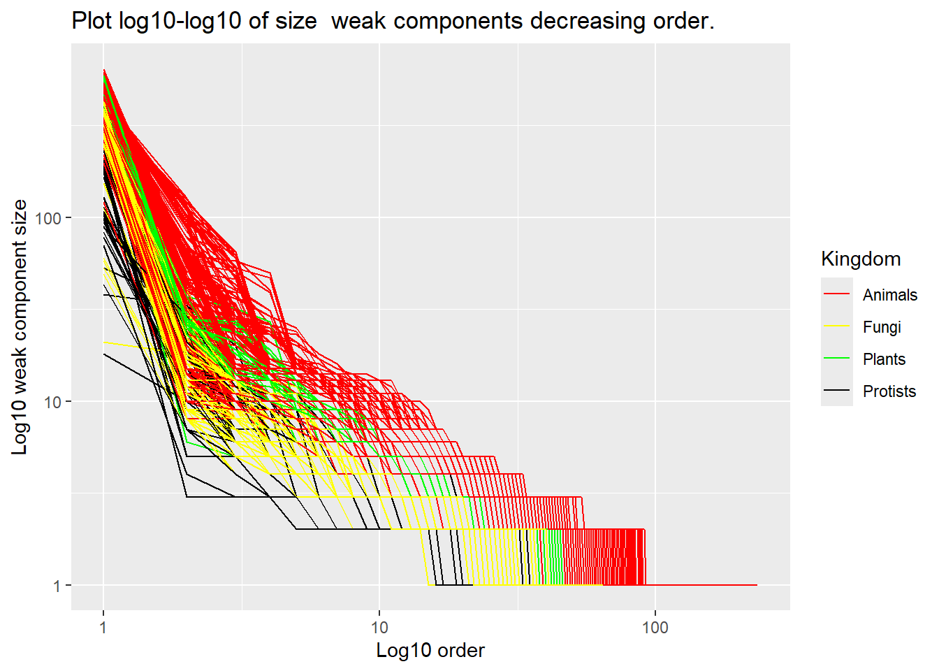
We can visualize the sizes of the weak components for each m-DAG, using colors to represent the different Kingdoms, also we scale the results by a log-log plot:
A table with the frequencies of the MBBs sizes displayed by Kingdom can be obtained as follows:
size_MBB_df_table= size_MBB_df %>%group_by(Kingdom,size) %>%summarise(n=n())table_MBB_size = size_MBB_df_table %>%pivot_wider(names_from = Kingdom, values_from = n, values_fill =list(n =0)) %>%arrange(size)knitr::kable(table_MBB_size, caption ="MBB Size: Frequency by Kingdom")%>%kable_styling(bootstrap_options ="striped", full_width =FALSE) %>%scroll_box(height ="300px", width ="100%")
MBB Size: Frequency by Kingdom
size
Animals
Fungi
Plants
Protists
1
408027
74872
109638
17773
2
7426
2464
2306
678
3
5087
464
758
303
4
2613
324
632
115
5
948
340
49
56
6
390
131
274
46
7
190
167
27
16
8
544
70
127
27
9
137
7
124
10
10
492
20
2
10
11
91
29
132
8
12
44
3
6
4
13
21
4
0
2
14
15
10
0
1
15
195
2
0
5
16
23
6
0
3
17
7
5
1
0
18
410
122
118
3
19
3
7
0
0
20
4
0
0
7
21
1
0
0
0
22
0
0
0
2
23
3
0
0
0
24
5
1
0
0
25
2
1
0
2
27
1
0
1
0
29
1
2
0
0
30
0
1
0
1
31
2
4
0
2
32
0
4
0
1
33
1
2
0
0
34
3
0
0
0
35
5
0
0
0
36
1
0
0
1
37
1
2
0
1
39
1
0
0
0
44
1
0
0
4
45
0
1
0
0
46
1
0
0
0
47
0
0
0
3
48
0
0
0
2
49
1
0
0
1
50
1
0
0
0
51
1
0
0
0
53
2
0
0
0
54
1
0
0
0
56
1
0
0
0
57
3
0
0
0
92
0
0
0
1
103
0
0
0
1
107
0
0
0
1
117
0
0
0
1
118
0
0
0
1
119
0
0
0
1
120
0
0
0
3
121
0
0
0
5
136
1
0
0
0
139
0
0
0
1
162
0
0
0
1
181
1
0
0
0
186
0
0
0
1
189
0
0
0
1
203
0
0
0
1
222
0
0
1
0
224
0
0
0
1
226
0
0
0
1
232
0
0
0
1
233
1
0
0
0
234
0
0
0
1
240
0
0
0
3
241
0
0
0
1
250
1
0
0
0
259
0
0
1
0
276
1
0
0
1
284
0
1
0
1
285
0
0
1
0
286
1
0
0
0
291
0
0
0
1
296
0
1
0
1
300
0
0
1
0
306
0
0
0
1
307
0
1
0
0
314
0
0
1
0
326
1
0
0
0
329
0
0
1
0
331
0
0
0
1
332
0
1
0
0
336
0
0
1
0
340
0
0
0
1
343
0
0
1
0
344
0
1
0
0
348
0
0
0
1
350
0
1
0
0
360
1
0
0
0
361
0
0
1
0
363
0
0
0
1
364
0
1
0
0
371
0
0
0
1
373
1
0
0
0
375
1
0
0
0
381
0
1
1
0
387
0
1
0
0
390
0
1
0
0
392
0
0
0
1
393
1
0
0
0
401
0
2
0
0
402
0
1
0
0
403
1
0
0
0
409
0
1
0
0
410
0
1
1
0
417
1
1
0
0
419
0
1
0
0
420
0
0
1
1
421
0
0
1
0
422
0
2
0
0
423
1
1
0
0
427
0
1
0
0
428
1
1
0
0
429
1
0
0
0
430
0
1
0
0
433
0
1
0
0
437
1
1
0
0
438
0
1
0
0
441
0
1
0
0
443
1
1
0
0
444
0
1
0
0
446
0
1
0
0
447
1
2
0
0
449
1
1
0
0
450
1
0
0
0
451
0
3
0
0
452
1
0
0
0
454
0
1
0
0
455
0
1
0
0
456
1
0
0
0
457
1
1
0
0
458
1
1
0
0
459
2
0
0
0
461
1
1
0
0
462
1
2
0
0
463
0
3
0
0
465
1
0
0
0
466
1
0
0
0
467
1
0
0
0
468
0
2
0
0
469
2
0
0
0
470
1
0
0
0
471
1
1
0
0
473
2
1
0
0
474
3
0
0
0
476
0
2
0
0
477
1
0
0
0
478
1
1
0
0
479
1
0
0
0
480
0
1
0
0
481
2
0
0
0
482
2
0
0
0
483
2
0
0
0
484
2
1
0
1
485
0
2
0
0
486
1
1
0
0
487
6
0
0
0
488
1
2
0
0
489
1
0
0
0
490
1
0
0
0
491
2
1
0
0
492
2
0
0
0
493
1
1
0
0
494
0
1
0
0
495
2
1
0
0
496
4
1
0
0
498
5
3
0
0
499
2
0
0
0
500
2
0
0
0
501
1
1
0
0
502
3
3
0
0
503
1
0
0
0
504
6
0
0
1
505
5
2
0
0
506
5
2
0
0
507
1
2
0
0
508
4
0
0
0
509
0
1
0
0
510
4
2
0
0
511
3
1
0
0
512
1
0
0
0
513
6
1
0
0
514
5
0
0
0
515
1
1
0
0
516
1
0
0
0
517
6
0
0
0
518
6
0
0
0
519
0
1
0
0
521
0
1
0
0
522
5
1
0
0
523
1
2
0
0
524
2
2
0
0
525
2
2
0
0
526
0
1
0
0
527
5
2
0
0
528
6
3
0
0
529
2
1
0
0
530
1
0
0
0
531
3
1
0
0
532
0
1
0
0
533
4
0
0
0
534
3
0
0
0
535
1
0
0
0
536
1
0
0
0
537
1
0
0
0
538
1
0
0
0
539
0
1
0
0
540
1
2
0
0
541
1
1
0
0
542
1
2
0
0
543
0
2
0
0
544
1
2
0
0
545
1
0
0
0
547
0
0
1
0
548
1
0
0
0
550
0
1
0
0
551
2
0
0
0
552
1
0
0
0
553
0
1
0
0
554
1
1
0
0
555
1
2
0
0
556
1
0
0
0
558
1
0
0
0
559
0
2
0
0
561
0
1
0
0
563
2
2
0
0
564
1
0
0
0
565
1
0
0
0
566
1
1
0
0
567
2
1
0
0
568
1
0
0
0
569
1
0
0
0
572
1
2
0
0
574
1
1
0
0
575
0
1
0
0
576
1
3
0
0
577
1
0
0
0
578
1
0
0
0
579
2
1
0
0
580
1
0
0
0
582
1
0
0
0
583
3
0
0
0
584
1
3
0
0
585
1
1
0
0
586
0
2
0
0
587
0
1
0
0
589
0
1
0
0
590
0
1
0
0
591
2
1
0
0
593
1
0
1
0
594
1
0
0
0
595
1
0
0
0
596
2
0
0
0
598
2
0
0
0
599
1
0
0
0
600
1
1
0
0
602
2
0
0
0
603
1
0
0
0
604
2
0
0
0
606
1
1
0
0
607
1
0
0
0
608
0
1
0
0
611
2
0
1
0
613
3
0
1
0
614
1
0
0
0
616
2
1
0
0
617
1
1
0
0
618
1
0
1
0
619
3
0
0
0
620
2
0
0
0
621
1
0
0
0
622
0
0
1
0
623
2
0
0
0
625
2
0
0
0
626
2
0
0
0
628
1
0
0
0
629
3
0
0
0
633
1
0
1
0
634
1
0
1
0
635
1
0
1
0
636
1
0
0
0
637
2
0
0
0
638
2
0
1
0
639
1
0
1
0
640
0
0
1
0
641
1
0
0
0
642
2
0
1
0
643
2
0
1
0
644
1
0
1
0
645
1
0
0
0
646
1
0
1
0
647
3
0
3
0
650
3
0
1
0
651
1
0
1
0
652
1
0
3
0
653
0
0
1
0
654
1
0
2
0
655
0
0
1
0
656
0
0
2
0
658
3
0
0
0
659
0
0
3
0
660
2
0
4
0
661
2
0
5
0
662
0
0
1
0
663
3
0
0
0
664
2
0
2
0
665
0
0
4
0
666
2
0
1
0
667
1
0
2
0
668
0
0
3
0
669
0
0
5
0
670
0
0
5
0
671
2
0
7
0
672
2
0
6
0
673
0
0
6
0
674
1
0
4
0
675
0
0
19
0
676
1
0
9
0
677
2
0
5
0
678
0
0
1
0
679
1
0
2
0
680
4
0
0
0
681
1
0
1
0
682
0
0
1
0
683
2
0
0
0
684
3
0
0
0
685
3
0
0
0
686
2
0
0
0
687
1
0
0
0
689
1
0
0
0
692
1
0
0
0
693
4
0
0
0
695
4
0
0
0
696
3
0
0
0
697
4
0
0
0
698
4
0
0
0
699
4
0
0
0
700
10
0
0
0
701
5
0
0
0
702
9
0
0
0
703
8
0
0
0
704
19
0
0
0
705
19
0
0
0
706
7
0
0
0
707
6
0
0
0
708
4
0
0
0
709
4
0
0
0
710
20
0
0
0
711
6
0
0
0
712
17
0
0
0
713
9
0
0
0
714
10
0
0
0
715
4
0
0
0
716
5
0
0
0
717
3
0
0
0
718
8
0
0
0
719
4
0
0
0
721
2
0
0
0
723
1
0
0
0
724
2
0
0
0
726
1
0
0
0
757
1
0
0
0
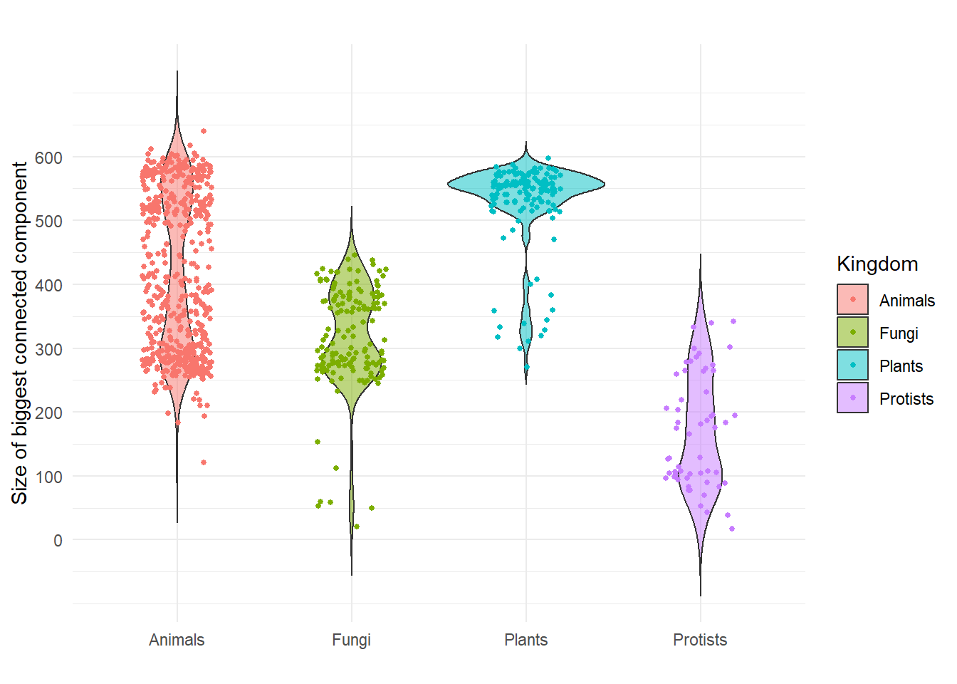
3.4.1 More statistics
h
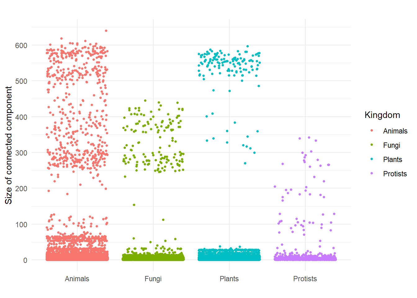
weak_components_size$Kingdom <-factor(weak_components_size$Kingdom)#weak_components_sizeg <-ggplot(weak_components_size) +xlab("") +# Eliminar el título del eje Xylab("Size of connected component") +# Etiqueta del eje Ygeom_jitter(aes(x = Kingdom, y = csize, color = Kingdom),size =1) +# Colorear puntos según 'Kingdom' y reducir el tamañoscale_y_continuous(breaks =seq(0, 640, by =100)) +# Escala del eje Y con saltos de 20theme_minimal() +# Tema minimalista con fondo blancoggtitle("") # Título del gráfico g
weak_components_size_max = weak_components_size %>%group_by(Organism) %>%summarise(csize =max(csize),Kingdom=first(Kingdom))# Crear el gráfico de violín con puntos jitterg <-ggplot(weak_components_size_max, aes(x = Kingdom, y = csize)) +geom_violin(aes(fill = Kingdom), trim =FALSE, alpha =0.5) +# Gráfico de violín con relleno por 'Kingdom' y sin recortargeom_jitter(aes(color = Kingdom), size =1, width =0.2) +# Puntos con jitter para evitar solapamientosxlab("") +# Eliminar el título del eje Xylab("Size of biggest connected component") +scale_y_continuous(breaks =seq(0, 640, by =100)) +theme_minimal() +# theme background whiteggtitle("") ##Size of the largest weakly connected component by Kingdom \n (Violin Plot with Jittered Points)# Mostrar el gráficog
Source Code
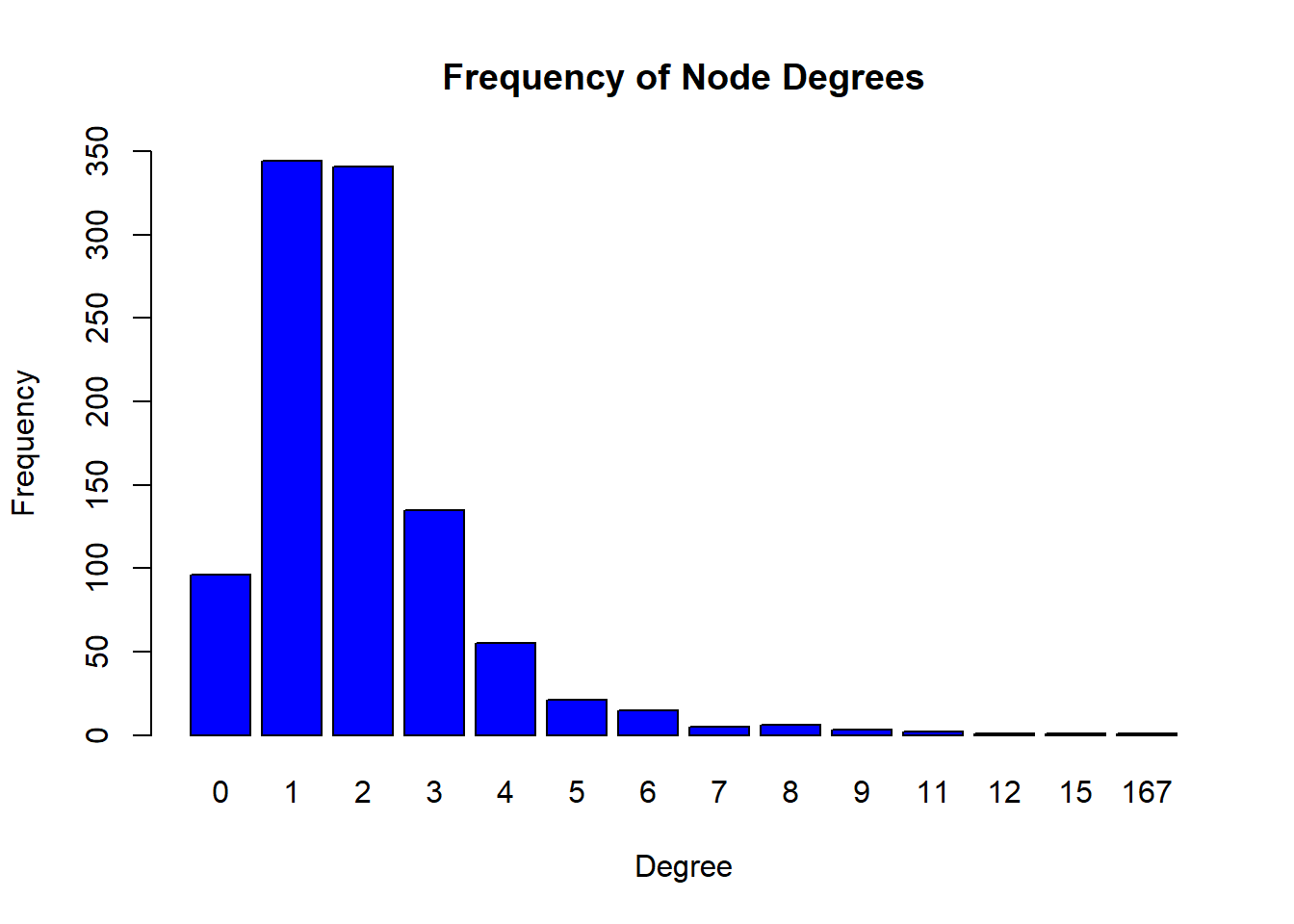
```{r include=FALSE,message=FALSE}knitr::opts_chunk$set(echo = TRUE, cache=TRUE, warning = FALSE, message = FALSE, out.width = "100%",cache.lazy=FALSE)pdf="TRUE"library(tidyverse)library(igraph)library(ComplexHeatmap)library(viridis)library(circlize)library(plotly)library(randomcoloR)library(factoextra)library(RColorBrewer)library(kableExtra)library(igraph)library(GGally)``````{r}gc()load(file='metadag_work_space.RData')gc()```# Metabolic GraphsWe present here some analysis examples of the metabolic graphs generated in GraphML format.## Metabolic graphs for each organismRead the individual metabolic graphs generated for Homo sapiens (KEGG id: hsa) in the directory(Individuals/hsa)```{r}experiment="0a845f74-826e-3b46-aed9-e7ecf74db262/"path_exp=paste0("data/",experiment)files_hsa=dir(paste0(path_exp,"Individuals/hsa"))files_hsa``````{r echo=FALSE}files_hsa=dir(paste0(path_exp,"Individuals/hsa"))# "plot mDAG pdf format",# "plot mDAG svg format",type_file=c("m-DAG GraphML format", "m-DAG pdf graphic", "m-DAG svg graphic", "csv file with the adjacency matrix of the m-DAG", "pdf graphic with the biggest conected component of the m-DAG", "svg graphic with the biggest conected component of the m-DAG ", "csv file with the node (MBBs) labels of the m-DAG", "csv file with all connected components of the m-DAG", "csv file with the adjacency matrix of the reaction graph", "csv file with the node (reactions) labels of the reaction graph", "reaction graph GraphML format", "reaction graph pdf graphic", "reaction graph svg graphic", "text summary file with the number of MBBs, reactions, etc. in the previous graphs")knitr::kable(data.frame(files_Individual_hsa=files_hsa, Description=type_file))```## Pan & core metabolic graphsPan and core metabolic graphs for every group were generated. For instance, one can read the pan and core metabolic graphs generated for the group Algae in the directory (Groups/Algae).```{r}files_Algae=dir(paste0(path_exp,"Groups/Algae"))files_Algae```The global core reaction graph, which is the core of all the organisms' reaction graphs in this Eukaryotes test, is empty.```{r graph_core_ALL}graph_core_RC=read.graph( paste0(path_exp, "Global/core/core_RC.graphml"), format = "graphml")summary(graph_core_RC)```The global core reaction graph has `r igraph::vcount(graph_core_RC)` vertex and `r igraph::ecount(graph_core_RC)` edges. It is an empty graph.The core reaction graph for the Algae group is:```{r fig.cap="Algae core reaction graph"}knitr::include_graphics( paste0(path_exp,"Groups/MSA_Cluster_3/core/MSA_Cluster_3_core_RC.pdf"))```The global core m-DAG, i.e., the core of all organisms in this example is empty.```{r}graph_core_mDAG=read.graph(paste0(path_exp,"Global/core/core_mDAG.graphml"),format ="graphml")summary(graph_core_mDAG)```The global core m-DAG has `r igraph::vcount(graph_core_mDAG)` vertex and `r igraph::ecount(graph_core_mDAG)` edges. It is an empty graph.The core metabolic DAG for the Algae group is:```{r fig.cap="Core m-DAG for Algae"}knitr::include_graphics(paste0(path_exp, "Groups/Algae/core/Algae_core_mDAG.pdf"))```The global pan reaction graph for the Animals Kingdom is:```{r}graph_pan_RC=read.graph(paste0(path_exp,"TaxonomyLevels/Kingdom/Animals/pan/Animals_pan_RC.graphml"),format ="graphml")summary(graph_pan_RC)```This pan reaction graph has `r igraph::vcount(graph_pan_RC)` nodes and `r igraph::ecount(graph_pan_RC)` edges.## Graph's topologyFrom the GraphML files, one can extract topological information. Some examples are as follows.The diagram below illustrates the distribution of node degrees for an m-DAG.```{r}graph_mDAG=read.graph(paste0(path_exp,"Individuals/hsa/hsa_mDAG.graphml"),format="graphml")summary(graph_mDAG)barplot(table(igraph::degree(graph_mDAG,mode="all")),ylim=c(0,350),col="blue",main="Frequency of Node Degrees",ylab="Frequency",xlab="Degree")```The connected components of every graph as well as the size of every connected component can be obtained as:```{r}compo=components(graph_mDAG,mode ="weak")str(compo)compo$csizek=which.max(compo$csize==max(compo$csize))ktable(compo$membership)vertex=which(compo$membership==k)length(vertex)Big_Component=induced_subgraph(graph_mDAG, vids=vertex)igraph::vcount(Big_Component)igraph::ecount(Big_Component)```And the plot of the bigger component of the m-DAG in Homo sapiens is:```{r fig.align='center',title="Bigger component of hsa mDAG"}knitr::include_graphics(paste0(path_exp, "Individuals/hsa/hsa_mDAG_biggerDAG.pdf"))``````{r}#path_exp="data/result_bb261b6e-95c6-3e39-b82b-b68eea80e30b/data/" list_names=dir(paste0(path_exp,"Individuals/"))list_names= list_names[-1] # filter 0000_RefPwlength(list_names) graphs_list=paste0(path_exp,"Individuals/", list_names,"/",list_names, "_MDAG.graphml")``````{r}knitr::include_graphics(paste0(path_exp,"Individuals/cang/cang_RC.pdf"))```## Graph statisticsThe number of connected component in each generated m-DAG with their frequency in the entire set of m-DAGs, can be obtained as follows:```{r ,warning=FALSE}read_mDAG=function(x) {DAG=read.graph(file=x, format="graphml")return(DAG)}mDAG_components=function(x) { sort(components(x,mode = "weak")$csize, decreasing=TRUE)}compo_list=lapply(graphs_list, FUN=function(x) { gg=read_mDAG(x) aux=list( mDAG_components=mDAG_components(gg), degree_count=igraph::degree(gg,mode="total")) return(aux)})names(compo_list)=list_namesn=max(sapply(compo_list,FUN=function(x) {length(x[[1]])}))nsize_compo_list=lapply(compo_list,FUN=function(x) { return(c(x[[1]],rep(NA,n-length(x[[1]]))))})aux=do.call(bind_cols,size_compo_list)weak_components_size=pivot_longer(aux,aaf:zvi,names_to="Organism", values_to="csize") %>% arrange(Organism,-csize)weak_components_size$index=rep(1:n,times=dim(aux)[2])weak_components_size=weak_components_size %>% left_join(meta_taxo,by="Organism") %>% filter(!is.na(Kingdom),!is.na(csize))weak_components_size_raw=weak_components_size``````{r ,warning=FALSE,cache=FALSE}Organism=names(compo_list)size_MBB=function(org){ #org="hsa" x=Results %>% filter(Organism==org) %>% select(!contains("_rev")) x=as.character(x[1,6:dim(x)[2]]) x=x[(!is.na(x))] x=x[x!="NA"] tt=data.frame(sort(table(x),decreasing=TRUE),org) names(tt)=c("MBB","size","Organism") return(tt)}size_list_raw= lapply(Organism,FUN=function(x) size_MBB(x))names(size_list_raw)=Organism``````{r ,warning=FALSE,cache=FALSE}size_MBB_df=do.call(rbind,size_list_raw)max(size_MBB_df$size)size_MBB_df=size_MBB_df %>% left_join(meta_taxo%>% select(Organism,Kingdom),by="Organism") %>% filter(!is.na(Kingdom))```We can visualize the sizes of the weak components for each m-DAG, using colors to represent the different Kingdoms, also we scale the results by a log-log plot:```{r}COLOR_KINGDOM=c("red","yellow","green","black")colors_kingdom=weak_components_size%>%select(Organism,Kingdom) %>%distinct()names(COLOR_KINGDOM)=sort(unique(colors_kingdom$Kingdom))p1<-ggplot(data=weak_components_size) +geom_line(mapping=aes(x=index,y=csize,group = Organism,color=Kingdom),na.rm=TRUE) +scale_x_continuous(trans="identity") +scale_y_continuous(trans="identity") +ylim(0,640)+ggtitle("Plot of weak components size decreasing order.")+ylab("Weak components size") +xlab("Order")+scale_color_manual(values =COLOR_KINGDOM[colors_kingdom$Kingdom])p2<-ggplot(data=weak_components_size) +geom_line(mapping=aes(x=index,y=csize,group = Organism,color=Kingdom),na.rm=TRUE) +scale_y_continuous(trans='log10') +scale_x_continuous(trans='log10') +scale_color_manual(values =COLOR_KINGDOM[colors_kingdom$Kingdom])+ggtitle("Plot log10-log10 of size weak components decreasing order.") +ylab("Log10 weak component size") +xlab("Log10 order")p1p2```A table with the frequencies of the weak connected components sizes, displayed by Kingdom, can be obtained as follows:```{r}aux=table(weak_components_size$csize,weak_components_size$Kingdom)table_wcc_size=tibble(Order=1:dim(aux)[1],Wcc_size=as.integer(unlist(dimnames(aux)[1])),Animals=aux[,1],Fungi=aux[,2],Plants=aux[,3],Protists=aux[,4])knitr::kable(table_wcc_size, caption ="Weak Connected Componet Size")%>%kable_styling(bootstrap_options ="striped", full_width =FALSE) %>%scroll_box(height ="300px", width ="100%")```A table with the frequencies of the MBBs sizes displayed by Kingdom can be obtained as follows:```{r}size_MBB_df_table= size_MBB_df %>%group_by(Kingdom,size) %>%summarise(n=n())table_MBB_size = size_MBB_df_table %>%pivot_wider(names_from = Kingdom, values_from = n, values_fill =list(n =0)) %>%arrange(size)knitr::kable(table_MBB_size, caption ="MBB Size: Frequency by Kingdom")%>%kable_styling(bootstrap_options ="striped", full_width =FALSE) %>%scroll_box(height ="300px", width ="100%")``````{r include=FALSE}write_csv(table_MBB_size,"table_MBB_size.csv")``````{r pasar_load, include=FALSE}save.image(file='metadag_work_space.RData')```### More statisticsh```{r}weak_components_size$Kingdom <-factor(weak_components_size$Kingdom)#weak_components_sizeg <-ggplot(weak_components_size) +xlab("") +# Eliminar el título del eje Xylab("Size of connected component") +# Etiqueta del eje Ygeom_jitter(aes(x = Kingdom, y = csize, color = Kingdom),size =1) +# Colorear puntos según 'Kingdom' y reducir el tamañoscale_y_continuous(breaks =seq(0, 640, by =100)) +# Escala del eje Y con saltos de 20theme_minimal() +# Tema minimalista con fondo blancoggtitle("") # Título del gráfico g``````{r}weak_components_size_max = weak_components_size %>%group_by(Organism) %>%summarise(csize =max(csize),Kingdom=first(Kingdom))# Crear el gráfico de violín con puntos jitterg <-ggplot(weak_components_size_max, aes(x = Kingdom, y = csize)) +geom_violin(aes(fill = Kingdom), trim =FALSE, alpha =0.5) +# Gráfico de violín con relleno por 'Kingdom' y sin recortargeom_jitter(aes(color = Kingdom), size =1, width =0.2) +# Puntos con jitter para evitar solapamientosxlab("") +# Eliminar el título del eje Xylab("Size of biggest connected component") +scale_y_continuous(breaks =seq(0, 640, by =100)) +theme_minimal() +# theme background whiteggtitle("") ##Size of the largest weakly connected component by Kingdom \n (Violin Plot with Jittered Points)# Mostrar el gráficog```