Lección 2 Descripción de la muestra de casos según sintomatología
Hubo:
745 infecciones asintomáticas (44.66%)
643 infecciones leves (38.55%)
280 infecciones graves (16.79%)
Síntomas=ordered(c("Asintomática", "Leve", "Grave"),levels=c("Asintomática", "Leve", "Grave"))
valor=as.vector(prop.table(table(Sint)))
data <- data.frame(Síntomas,valor)

ggplot(data, aes(x=Síntomas, y=valor,fill=Síntomas)) +
  geom_bar(stat="identity")+
  xlab("")+
  ylab("")+
  scale_fill_brewer(palette = "Dark2") +
  theme(legend.position="none")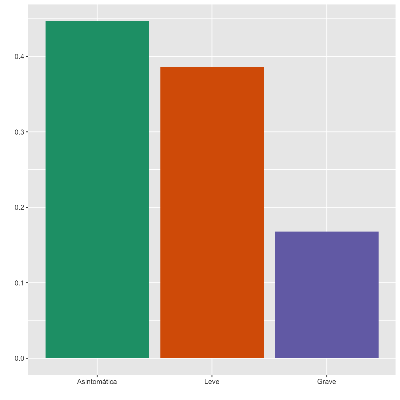
Figura 2.1:
Trim=Casos$Trim.Diag
NA_T=length(Trim[is.na(Trim)])
NA_S=length(Sint[is.na(Sint)])

DF=data.frame(Trimestre=Trim,Síntomas=Sint)
taula=table(DF)[,1:3]
proptaula=round(100*prop.table(table(DF)),2)[,1:3]

EEExt=cbind(c(as.vector(taula[,1]),sum(taula[,1])),
            c(as.vector(proptaula[,1]), round(100*sum(taula[,1])/n_I,2)),
            c(as.vector(taula[,2]),sum(taula[,2])),
            c(as.vector(proptaula[,2]), round(100*sum(taula[,2])/n_I,2)),
            c(as.vector(taula[,3]),sum(taula[,3])),
            c(as.vector(proptaula[,3]), round(100*sum(taula[,3])/n_I,2))
            )
rownames(EEExt)=c("1er trimestre", "2o trimestre", "3er trimestre","Total")
colnames(EEExt)=Columnes.Sint

EEExt %>%
  kbl() %>%
  kable_styling() %>%
scroll_box(width="100%", box_css="border: 0px;")| Asintomáticas (N) | Asintomáticas (%) | Leves (N) | Leves (%) | Graves (N) | Graves (%) | |
|---|---|---|---|---|---|---|
| 1er trimestre | 14 | 0.84 | 67 | 4.02 | 10 | 0.60 |
| 2o trimestre | 45 | 2.70 | 183 | 10.97 | 57 | 3.42 |
| 3er trimestre | 686 | 41.13 | 393 | 23.56 | 213 | 12.77 |
| Total | 745 | 44.66 | 643 | 38.55 | 280 | 16.79 |
Síntomas=ordered(rep(c("Asintomática", "Leve", "Grave"), each=3),levels=c("Asintomática", "Leve", "Grave"))
Grupo=rep(c("1er trimestre", "2o trimestre", "3er trimestre") , 3)
valor=as.vector(prop.table(taula, margin=1))
data <- data.frame(Grupo,Síntomas,valor)

ggplot(data, aes(fill=Síntomas, y=valor, x=Grupo)) +
  geom_bar(position="dodge", stat="identity")+
  xlab("Trimestre de infección")+
  ylab("")+
scale_fill_brewer(palette = "Dark2") 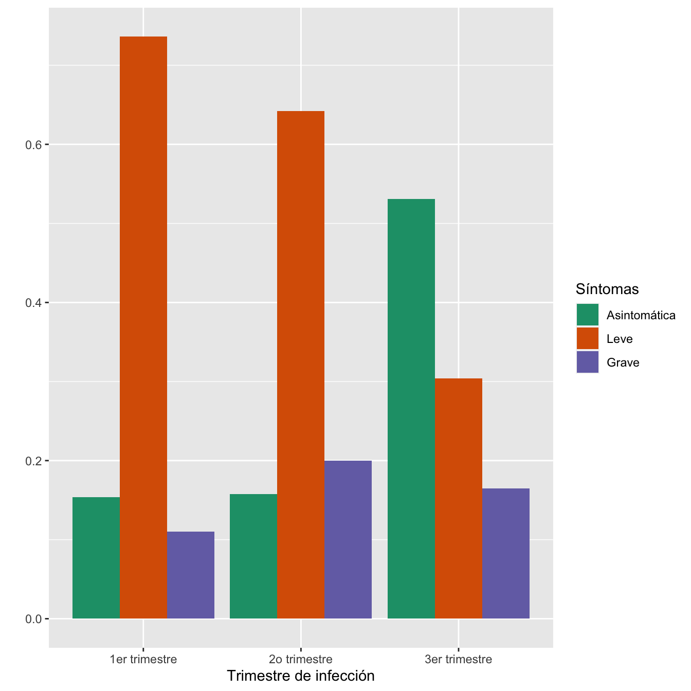
Figura 2.2:
2.1 Antecedentes maternos
2.1.1 Edades
I=Casos$Edad._años_
DF=data.frame(Edad=I,Sint=Casos$SINTOMAS_DIAGNOSTICO)


DF %>%
  ggplot( aes(x=Sint, y=Edad, fill=Sint)) +
    geom_violin(width=1) +
    geom_boxplot(width=0.1, color="black", alpha=0.2,outlier.fill="black",
               outlier.size=1) +
    theme(
      legend.position="none",
      plot.title=element_text(size=11)
    ) +
    xlab("")+
  ylab("Edades (años)")+
 scale_fill_brewer(palette="Dark2")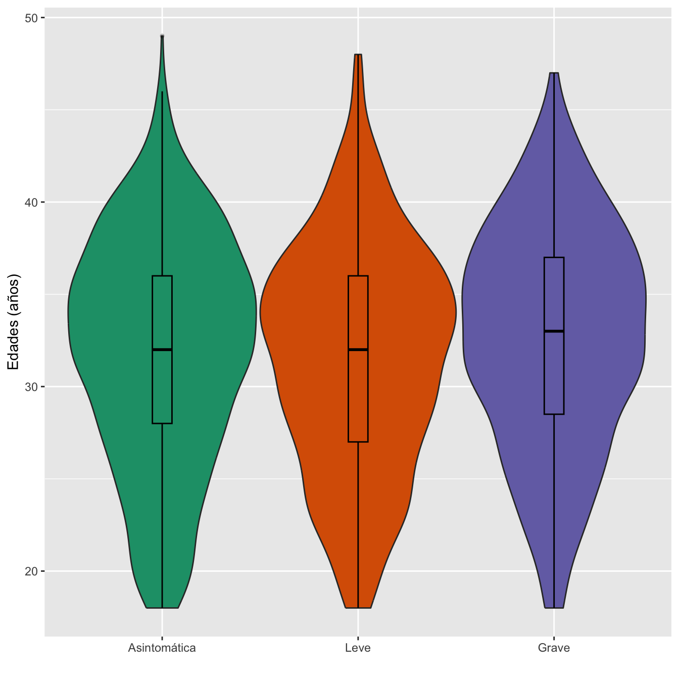
I1=I[Casos$SINTOMAS_DIAGNOSTICO=="Asintomática"]
I2=I[Casos$SINTOMAS_DIAGNOSTICO=="Leve"]
I3=I[Casos$SINTOMAS_DIAGNOSTICO=="Grave"]

Dades=rbind(c(round(min(I1,na.rm=TRUE),1),round(max(I1,na.rm=TRUE),1), round(mean(I1,na.rm=TRUE),1),round(median(I1,na.rm=TRUE),1),round(quantile(I1,c(0.25,0.75),na.rm=TRUE),1), round(sd(I1,na.rm=TRUE),1)),
            c(round(min(I2,na.rm=TRUE),1),round(max(I2,na.rm=TRUE),1), round(mean(I2,na.rm=TRUE),1),round(median(I2,na.rm=TRUE),1),round(quantile(I2,c(0.25,0.75),na.rm=TRUE),1), round(sd(I2,na.rm=TRUE),1)),
            c(round(min(I3,na.rm=TRUE),1),round(max(I3,na.rm=TRUE),1), round(mean(I3,na.rm=TRUE),1),round(median(I3,na.rm=TRUE),1),round(quantile(I3,c(0.25,0.75),na.rm=TRUE),1), round(sd(I3,na.rm=TRUE),1)))

colnames(Dades)=c("Edad mínima","Edad máxima","Edad  media", "Edad  mediana", "1er cuartil", "3er cuartil", "Desv. típica")
rownames(Dades)=c("Asintomática", "Leve","Grave")

Dades %>%
  kbl() %>%
  kable_styling() %>%
scroll_box(width="100%", box_css="border: 0px;")| Edad mínima | Edad máxima | Edad media | Edad mediana | 1er cuartil | 3er cuartil | Desv. típica | |
|---|---|---|---|---|---|---|---|
| Asintomática | 18 | 49 | 31.9 | 32 | 28.0 | 36 | 6.2 |
| Leve | 18 | 48 | 31.5 | 32 | 27.0 | 36 | 6.1 |
| Grave | 18 | 47 | 32.6 | 33 | 28.5 | 37 | 6.0 |
Ajuste de las edades maternas a distribuciones normales: test de Shapiro-Wilks, p-valores \(10^{-7}\), \(10^{-4}\) y 0.0126, respectivamente
Edades medias: test de Kruskal-Wallis, p-valor 0.0445112
Desviaciones típicas: test de Fligner-Killeen, p-valor 0.91
Contrastes post hoc por parejas
Contraste=c("Asíntomatica vs Leve","Asíntomatica vs Grave", "Leve vs Grave")

pvals=round(3*c(t.test(I1,I2,var.equal=TRUE)$p.value, t.test(I1,I3,var.equal=TRUE)$p.value,
            t.test(I2,I3,var.equal=TRUE)$p.value),4)
dades=data.frame(Contraste=Contraste,"p-valor"=pvals)
dades %>%
  kbl() %>%
  kable_styling() %>%
scroll_box(width="100%", box_css="border: 0px;")| Contraste | p.valor |
|---|---|
| Asíntomatica vs Leve | 0.9667 |
| Asíntomatica vs Grave | 0.2546 |
| Leve vs Grave | 0.0414 |
En tablas como la que sigue:
p-valor: El p-valor del test \(\chi^2\) de si la distribución de la fila correspondiente en casos sintomáticos es la misma que la del global de la muestra de casos, ajustado por Bonferroni cuando haya más de 2 filas
Tipo: El tipo de test \(\chi^2\), paramétrico, siempre que es posible, o Montecarlo, cuando no se dan las condiciones necesarias para que tenga sentido efectuar el test paramétrico
I.cut=cut(I,breaks=c(0,30,40,100),labels=c("18-30","31-40",">40"))
Tabla.DMCasosm(I.cut, c("18-30", "31-40", ">40"))| Asintomáticas (N) | Asintomáticas (%) | Leves (N) | Leves (%) | Graves (N) | Graves (%) | p-valor | Tipo | |
|---|---|---|---|---|---|---|---|---|
| 18-30 | 281 | 37.9 | 273 | 42.5 | 93 | 33.3 | 0.070056 | Paramétrico |
| 31-40 | 412 | 55.5 | 326 | 50.8 | 163 | 58.4 | 0.186490 | Paramétrico |
| >40 | 49 | 6.6 | 43 | 6.7 | 23 | 8.2 | 1.000000 | Paramétrico |
| Datos perdidos | 3 | 1 | 1 |
Síntomas=ordered(rep(c("Asintomática", "Leve", "Grave"), each=3),levels=c("Asintomática", "Leve", "Grave"))
Grupo=ordered(rep(c("18-30","31-40",">40") , 3),levels=c("18-30","31-40",">40"))

taula=table(data.frame(Edad=I.cut,Síntomas=Sint))
valor=as.vector(prop.table(taula, margin=1))
data <- data.frame(Grupo,Síntomas,valor)

ggplot(data, aes(fill=Síntomas, y=valor, x=Grupo)) +
  geom_bar(position="dodge", stat="identity")+
  xlab("Edad")+
  ylab("")+
scale_fill_brewer(palette = "Dark2") 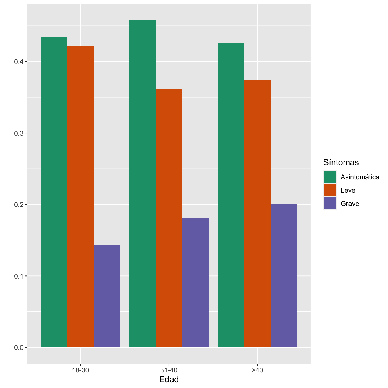
Figura 2.3:
- Asociación entre los grupos de sintomatología y las franjas de edad: test \(\chi^2\), p-valor 0.092
2.1.2 Etnia
I=Casos$Etnia
I[I=="Asia"]="Asiática"
I=factor(I)
Tabla.DMCasosm(I,c("Árabe", "Asiática", "Blanca", "Latinoamericana","Negra"))| Asintomáticas (N) | Asintomáticas (%) | Leves (N) | Leves (%) | Graves (N) | Graves (%) | p-valor | Tipo | |
|---|---|---|---|---|---|---|---|---|
| Árabe | 81 | 10.9 | 45 | 7.0 | 15 | 5.4 | 0.023462 | Paramétrico |
| Asiática | 26 | 3.5 | 11 | 1.7 | 12 | 4.3 | 0.248939 | Paramétrico |
| Blanca | 467 | 62.8 | 341 | 53.2 | 116 | 41.7 | 0.000000 | Paramétrico |
| Latinoamericana | 144 | 19.4 | 229 | 35.7 | 132 | 47.5 | 0.000000 | Paramétrico |
| Negra | 26 | 3.5 | 15 | 2.3 | 3 | 1.1 | 0.418159 | Paramétrico |
| Datos perdidos | 1 | 2 | 2 |
Síntomas=ordered(rep(c("Asintomática", "Leve", "Grave"), each=5),levels=c("Asintomática", "Leve", "Grave"))
Grupo=ordered(rep(c("Árabe", "Asiática", "Blanca", "Latinoamericana","Negra") , 3),levels=c("Árabe", "Asiática", "Blanca", "Latinoamericana","Negra"))

taula=table(data.frame(Etnia=I,Síntomas=Sint))
valor=as.vector(prop.table(taula, margin=1))
data <- data.frame(Grupo,Síntomas,valor)

ggplot(data, aes(fill=Síntomas, y=valor, x=Grupo)) +
  geom_bar(position="dodge", stat="identity")+
  xlab("Etnia")+
  ylab("")+
scale_fill_brewer(palette = "Dark2") 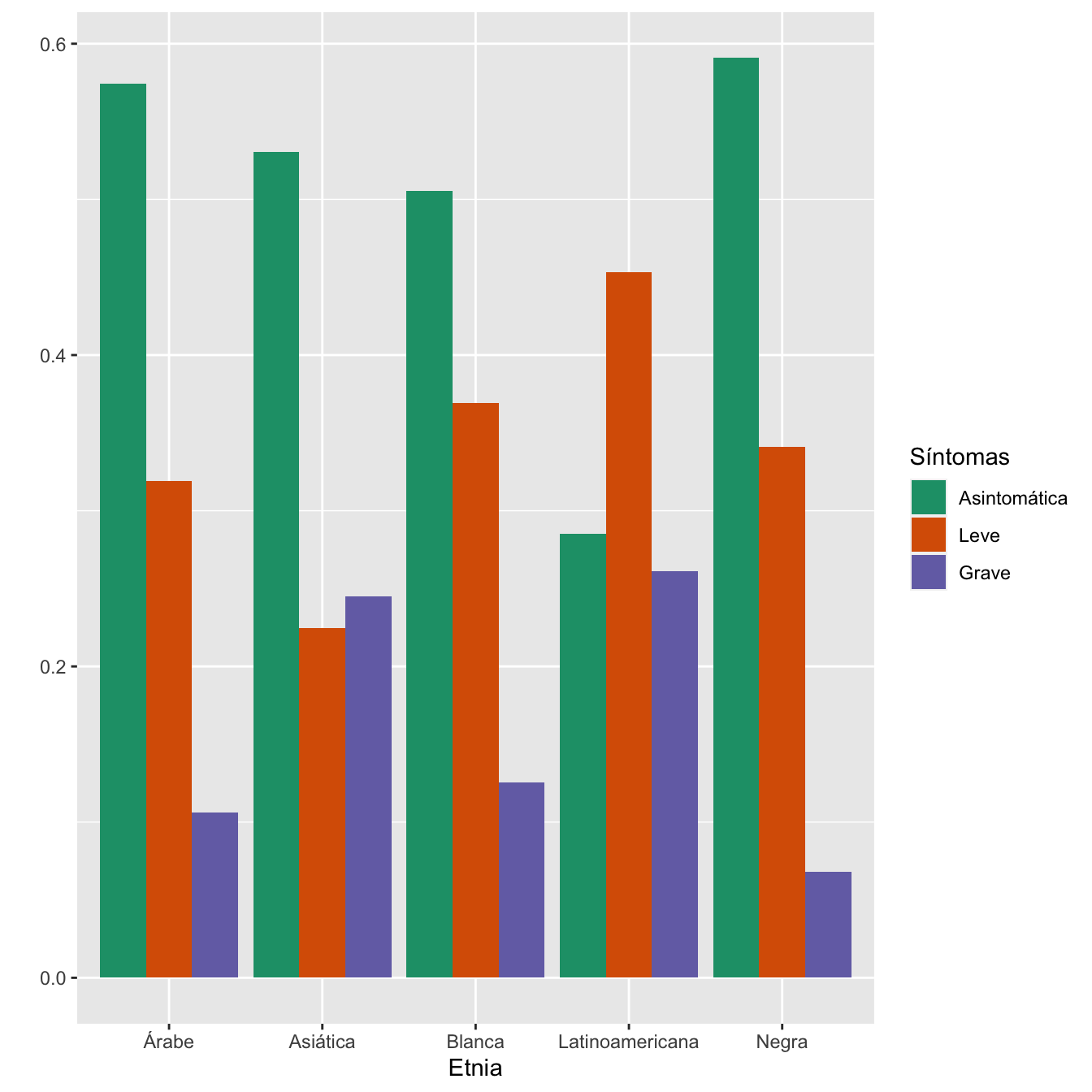
Figura 2.4:
- Asociación entre los grupos de sintomatología y las etnias: test \(\chi^2\), p-valor \(4\times 10^{-18}\)
2.1.3 Hábito tabáquico
taula=table(data.frame(Casos$FUMADORA_CAT,Sint))[c(2,1) ,1:3]
Tabla.DMCasos(Casos$FUMADORA_CAT,"Fumadoras", "No fumadoras")| Asintomáticas (N) | Asintomáticas (%) | Leves (N) | Leves (%) | Graves (N) | Graves (%) | p-valor | Tipo | |
|---|---|---|---|---|---|---|---|---|
| Fumadoras | 72 | 10.1 | 61 | 9.7 | 20 | 7.5 | 0.470802 | Paramétrico |
| No fumadoras | 640 | 89.9 | 569 | 90.3 | 245 | 92.5 | ||
| Datos perdidos | 33 | 13 | 15 |
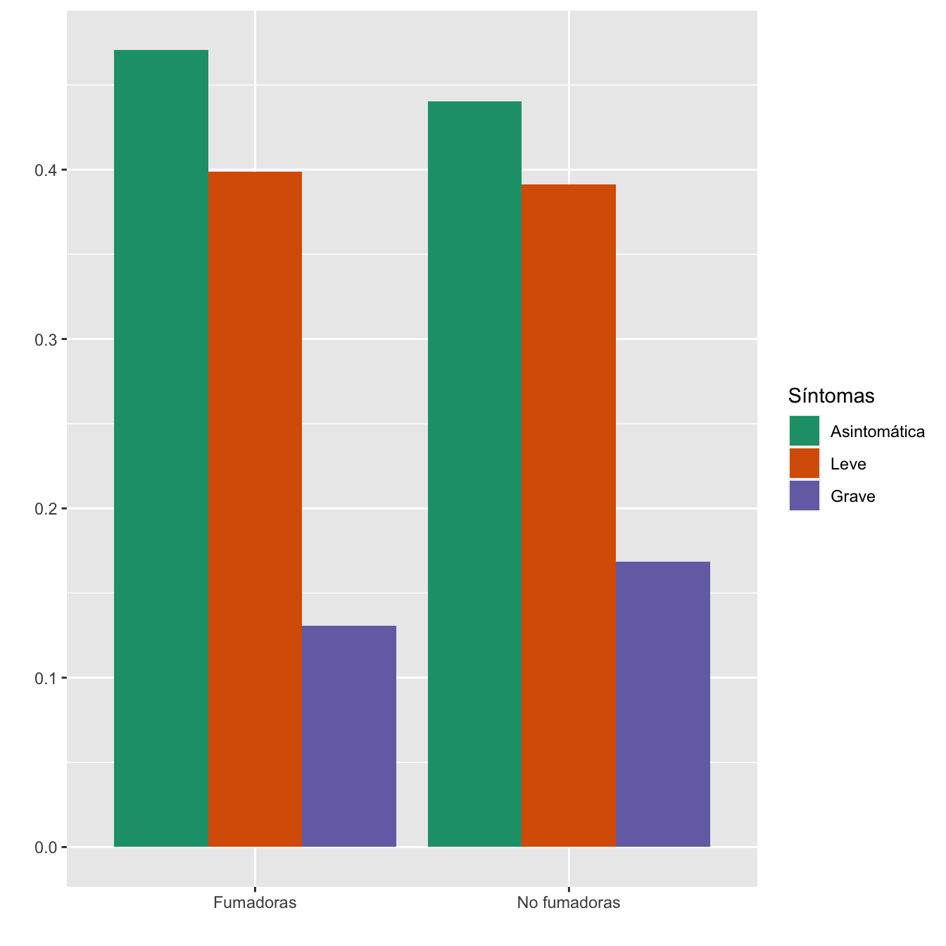
Figura 2.5:
- Potencia del test: 0.179
2.1.4 Obesidad
taula=table(data.frame(Casos$Obesidad,Sint))[c(2,1) ,1:3]
Tabla.DMCasos(Casos$Obesidad,"Obesas", "No obesas")| Asintomáticas (N) | Asintomáticas (%) | Leves (N) | Leves (%) | Graves (N) | Graves (%) | p-valor | Tipo | |
|---|---|---|---|---|---|---|---|---|
| Obesas | 118 | 15.8 | 119 | 18.5 | 68 | 24.3 | 0.007627 | Paramétrico |
| No obesas | 627 | 84.2 | 524 | 81.5 | 212 | 75.7 | ||
| Datos perdidos | 0 | 0 | 0 |
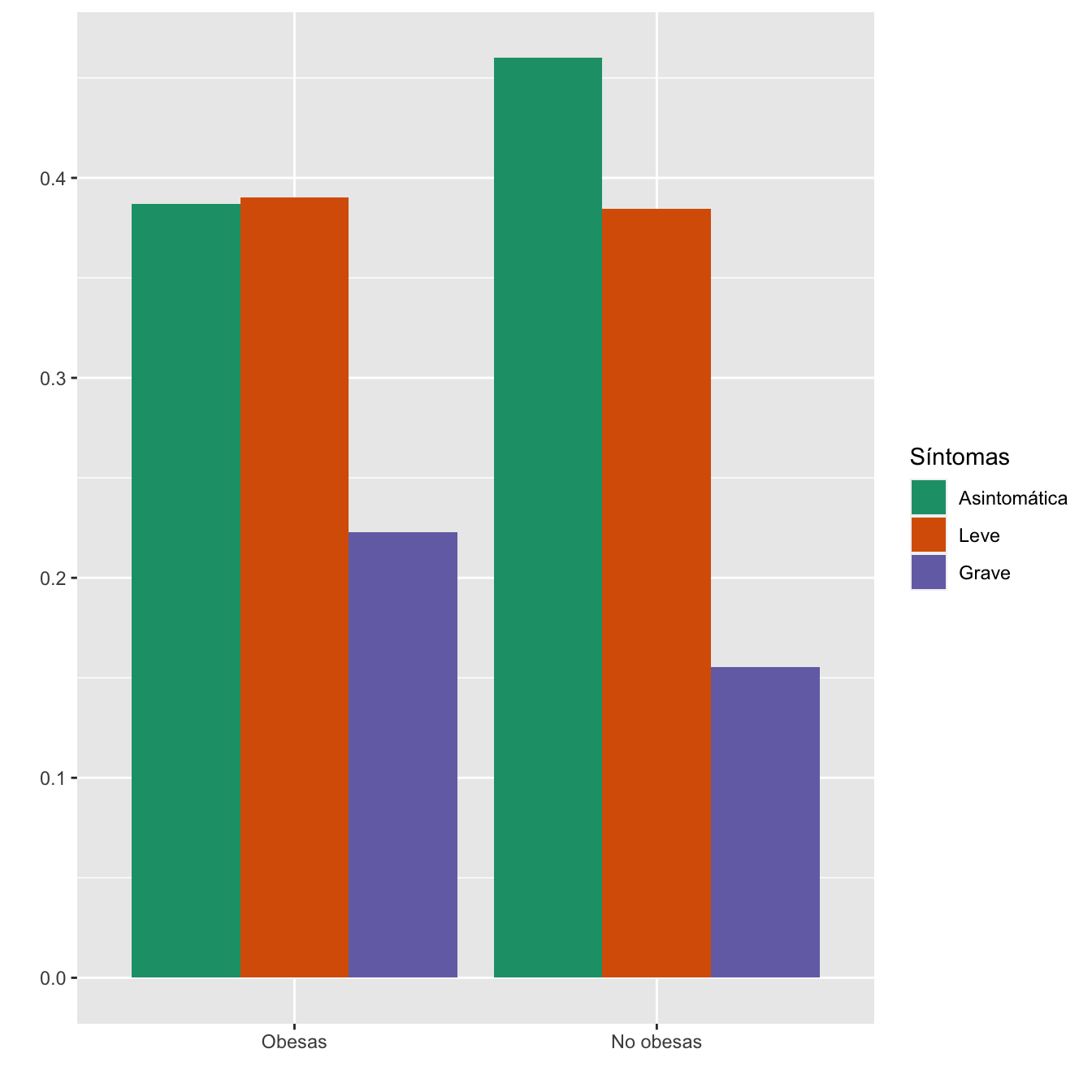
Figura 2.6:
- Potencia del test: 0.805
2.1.5 Hipertensión pregestacional
taula=table(data.frame(Casos$Hipertensión.pregestacional,Sint))[c(2,1) ,1:3]
Tabla.DMCasos(Casos$Hipertensión.pregestacional,"HTA", "No HTA")| Asintomáticas (N) | Asintomáticas (%) | Leves (N) | Leves (%) | Graves (N) | Graves (%) | p-valor | Tipo | |
|---|---|---|---|---|---|---|---|---|
| HTA | 11 | 1.5 | 7 | 1.1 | 7 | 2.5 | 0.267573 | Montecarlo |
| No HTA | 734 | 98.5 | 636 | 98.9 | 273 | 97.5 | ||
| Datos perdidos | 0 | 0 | 0 |
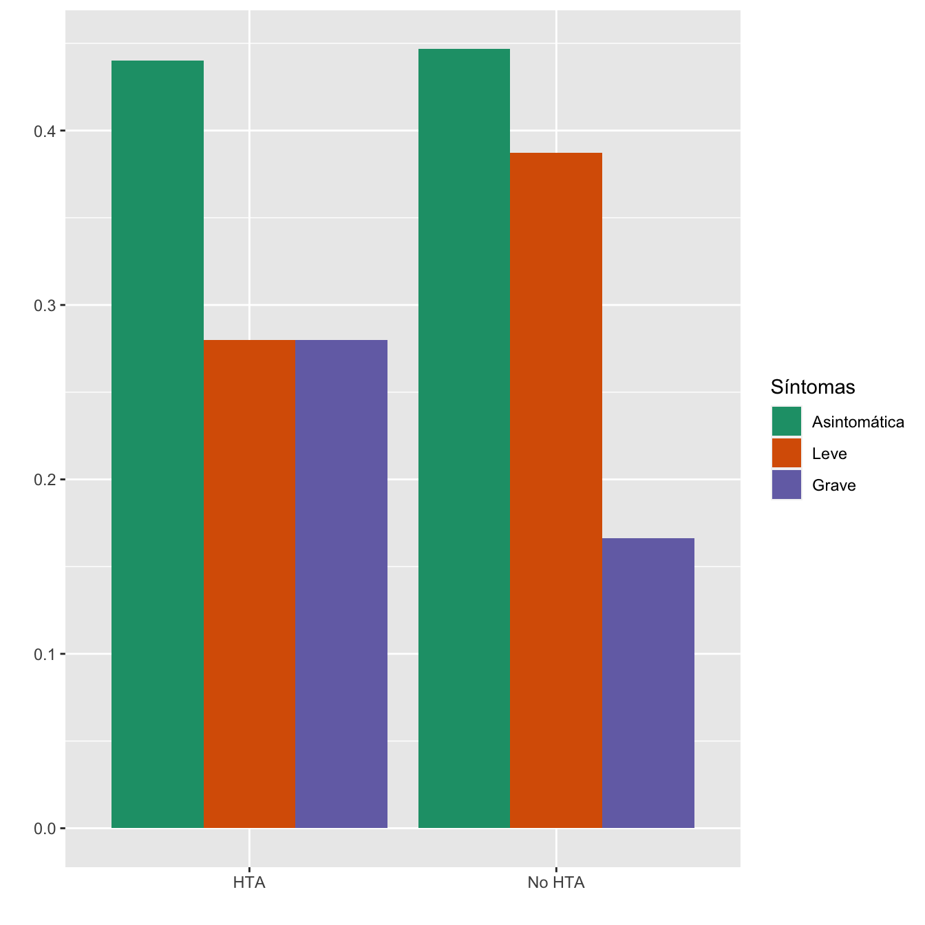
Figura 2.7:
- Potencia del test: 0.287
2.1.6 Diabetes
taula=table(data.frame(Casos$DIABETES,Sint))[c(2,1) ,1:3]
Tabla.DMCasos(Casos$DIABETES,"DM", "No DM")| Asintomáticas (N) | Asintomáticas (%) | Leves (N) | Leves (%) | Graves (N) | Graves (%) | p-valor | Tipo | |
|---|---|---|---|---|---|---|---|---|
| DM | 12 | 1.6 | 15 | 2.3 | 8 | 2.9 | 0.402704 | Paramétrico |
| No DM | 733 | 98.4 | 628 | 97.7 | 272 | 97.1 | ||
| Datos perdidos | 0 | 0 | 0 |
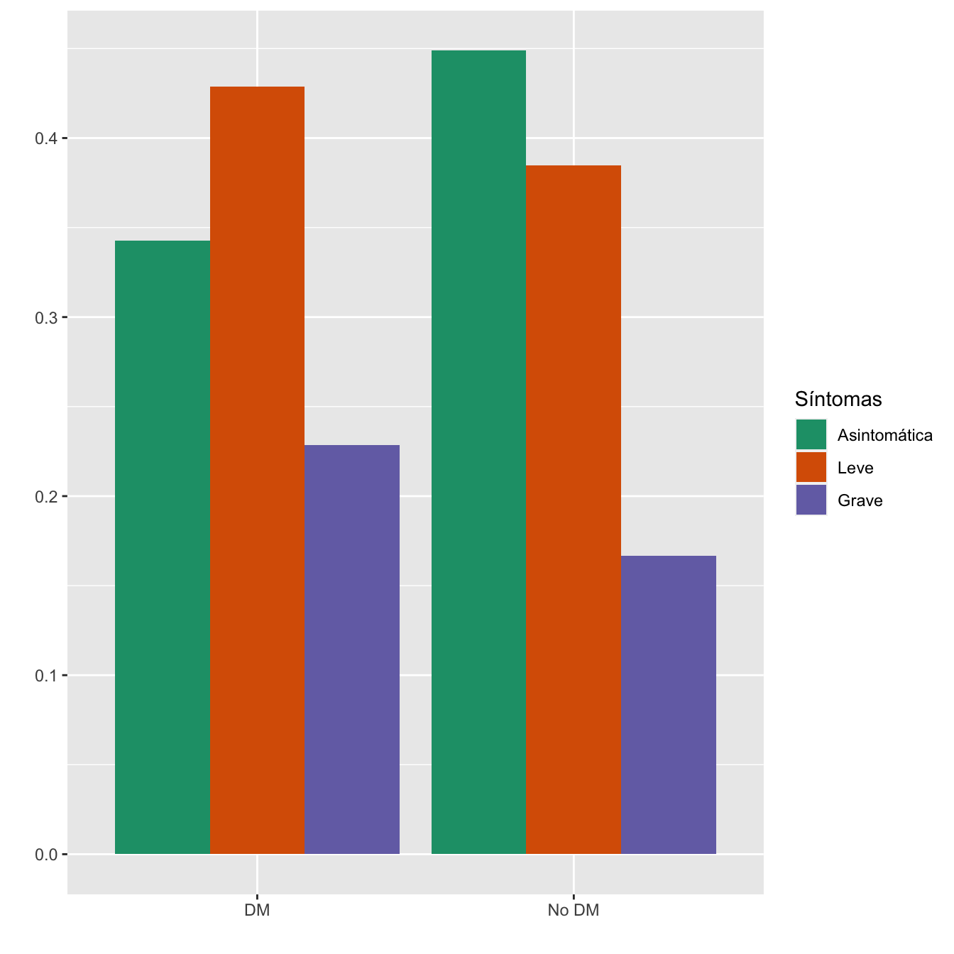
Figura 2.8:
- Potencia del test: 0.208
2.1.7 Cardiopatía
taula=table(data.frame(Casos$Enfermedad.cardiaca.crónica,Sint))[c(2,1) ,1:3]
Tabla.DMCasos(Casos$Enfermedad.cardiaca.crónica,"ECC", "No ECC")| Asintomáticas (N) | Asintomáticas (%) | Leves (N) | Leves (%) | Graves (N) | Graves (%) | p-valor | Tipo | |
|---|---|---|---|---|---|---|---|---|
| ECC | 6 | 0.8 | 7 | 1.1 | 6 | 2.1 | 0.187581 | Montecarlo |
| No ECC | 739 | 99.2 | 636 | 98.9 | 274 | 97.9 | ||
| Datos perdidos | 0 | 0 | 0 |
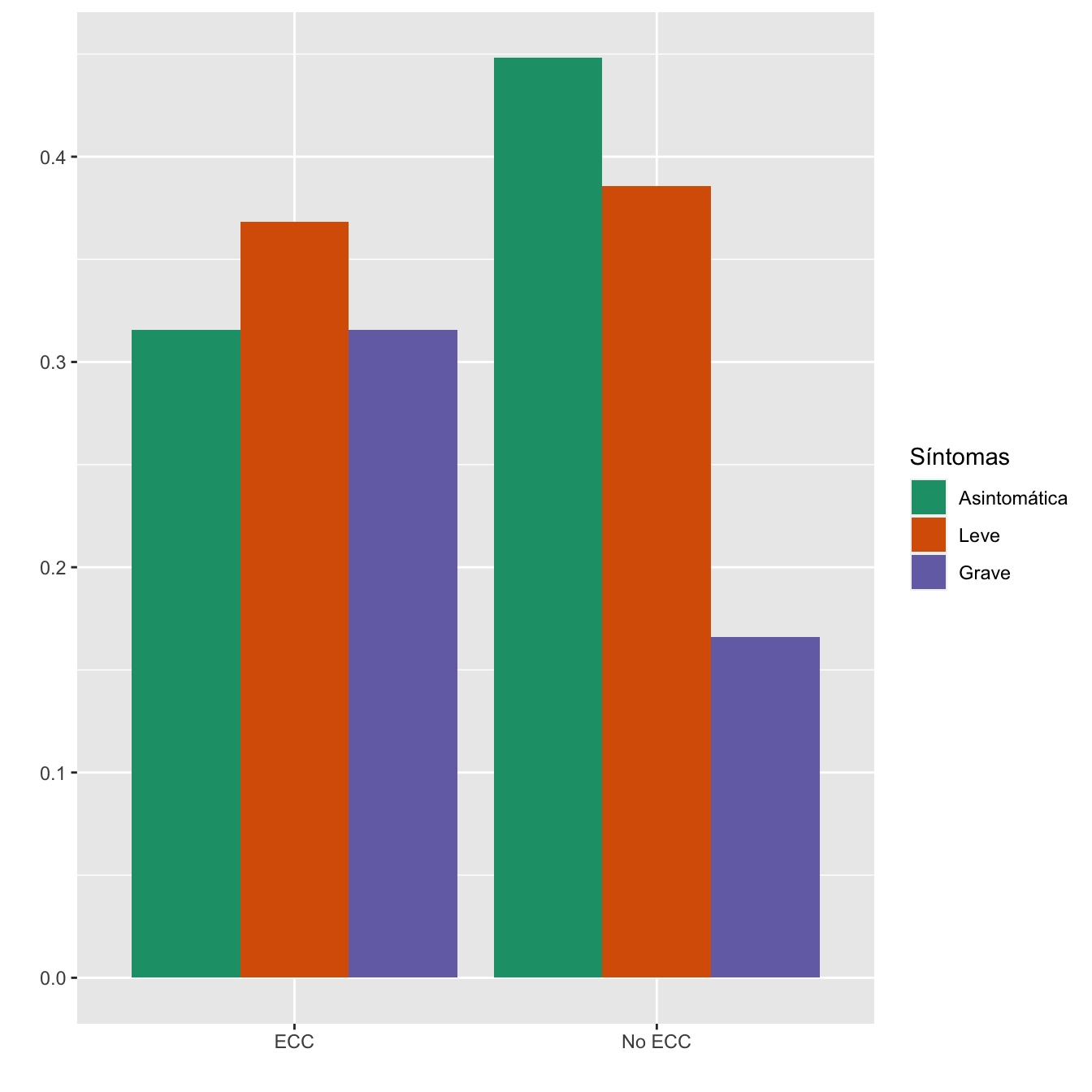
Figura 2.9:
- Potencia del test: 0.346
2.1.8 Enfermedad pulmonar crónica
INA=Casos$Enfermedad.pulmonar.crónica.no.asma
IA=Casos$Diagnóstico.clínico.de.Asma
I.EPC=rep(NA,length(Sint))
for (i in 1:length(Sint)){I.EPC[i]=max(INA[i],IA[i],na.rm=TRUE)}
taula=table(data.frame(I.EPC,Sint))[c(2,1) ,1:3]
Tabla.DMCasos(I.EPC,"EPC", "No EPC")| Asintomáticas (N) | Asintomáticas (%) | Leves (N) | Leves (%) | Graves (N) | Graves (%) | p-valor | Tipo | |
|---|---|---|---|---|---|---|---|---|
| EPC | 21 | 2.8 | 40 | 6.2 | 13 | 4.6 | 0.008846 | Paramétrico |
| No EPC | 724 | 97.2 | 603 | 93.8 | 267 | 95.4 | ||
| Datos perdidos | 0 | 0 | 0 |
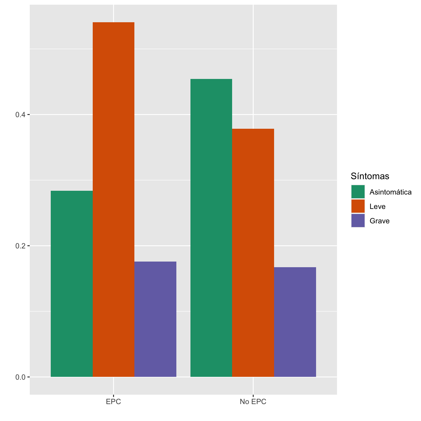
Figura 2.10:
- Potencia del test: 0.792
2.1.9 Gestación múltiple
taula=table(data.frame(Casos$Gestación.Múltiple,Sint))[c(2,1) ,1:3]
Tabla.DMCasos(Casos$Gestación.Múltiple,"Gestación múltiple", "Gestación única")| Asintomáticas (N) | Asintomáticas (%) | Leves (N) | Leves (%) | Graves (N) | Graves (%) | p-valor | Tipo | |
|---|---|---|---|---|---|---|---|---|
| Gestación múltiple | 8 | 1.1 | 17 | 2.6 | 6 | 2.1 | 0.090115 | Paramétrico |
| Gestación única | 737 | 98.9 | 626 | 97.4 | 274 | 97.9 | ||
| Datos perdidos | 0 | 0 | 0 |
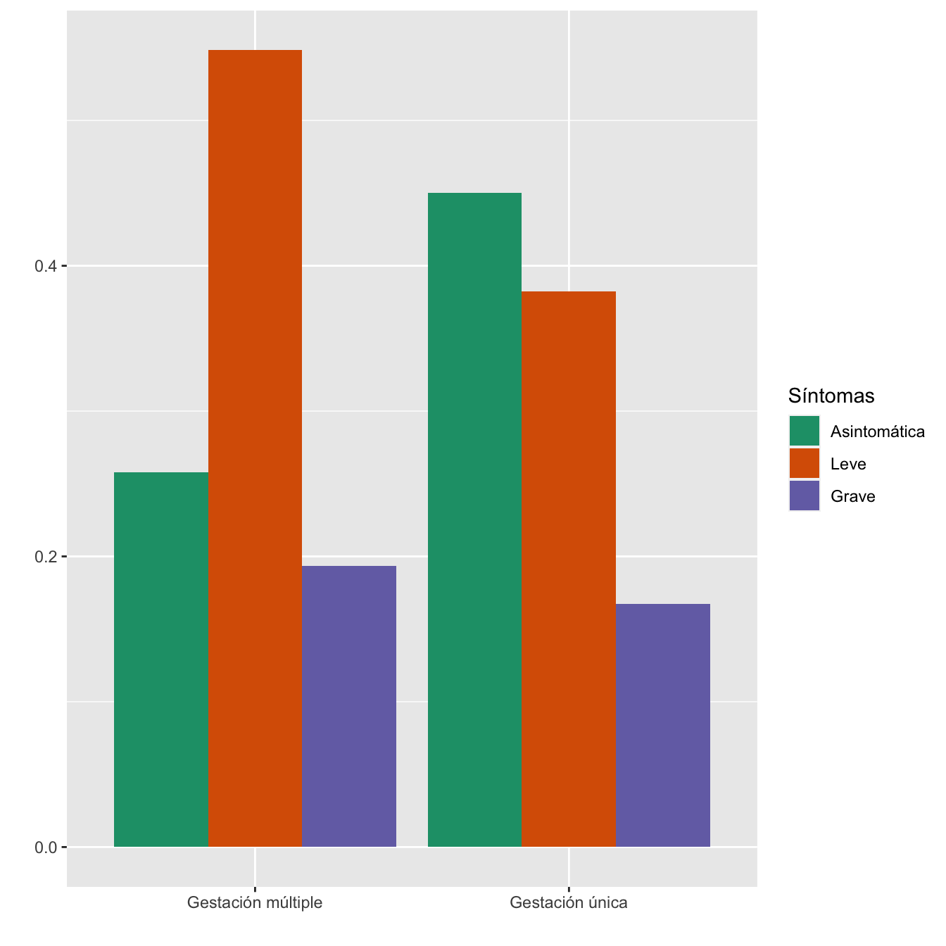
Figura 2.11:
- Potencia del test: 0.488
2.1.10 Paridad
taula=table(data.frame(Casos$NULIPARA,Sint))[c(2,1) ,1:3]
Tabla.DMCasos(Casos$NULIPARA, "Nulípara","Multípara")| Asintomáticas (N) | Asintomáticas (%) | Leves (N) | Leves (%) | Graves (N) | Graves (%) | p-valor | Tipo | |
|---|---|---|---|---|---|---|---|---|
| Nulípara | 275 | 37.4 | 250 | 39.1 | 81 | 29.1 | 0.013405 | Paramétrico |
| Multípara | 460 | 62.6 | 389 | 60.9 | 197 | 70.9 | ||
| Datos perdidos | 10 | 4 | 2 |
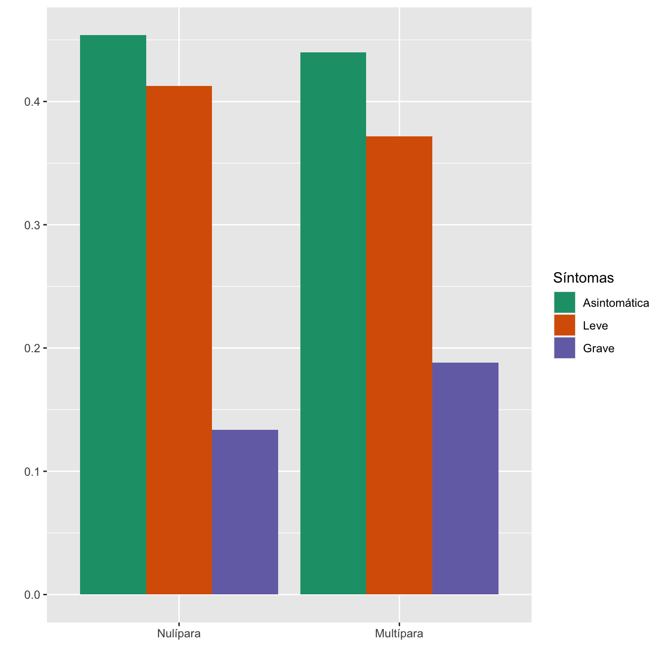
Figura 2.12:
- Potencia del test: 0.752
2.2 Desenlaces
2.2.1 Anomalía congénita
taula=table(data.frame(Casos$Diagnóstico.de.malformación.ecográfica._.semana.20._,Sint))[c(2,1) ,1:3]
Tabla.DMCasos(Casos$Diagnóstico.de.malformación.ecográfica._.semana.20._,"Anomalías congénitas", "No anomalías congénitas")| Asintomáticas (N) | Asintomáticas (%) | Leves (N) | Leves (%) | Graves (N) | Graves (%) | p-valor | Tipo | |
|---|---|---|---|---|---|---|---|---|
| Anomalías congénitas | 11 | 1.5 | 14 | 2.2 | 3 | 1.1 | 0.49795 | Montecarlo |
| No anomalías congénitas | 709 | 98.5 | 617 | 97.8 | 259 | 98.9 | ||
| Datos perdidos | 25 | 12 | 18 |
Barplot.DGS(Casos$Diagnóstico.de.malformación.ecográfica._.semana.20._,"Anomalías congénitas", "No anomalías congénitas")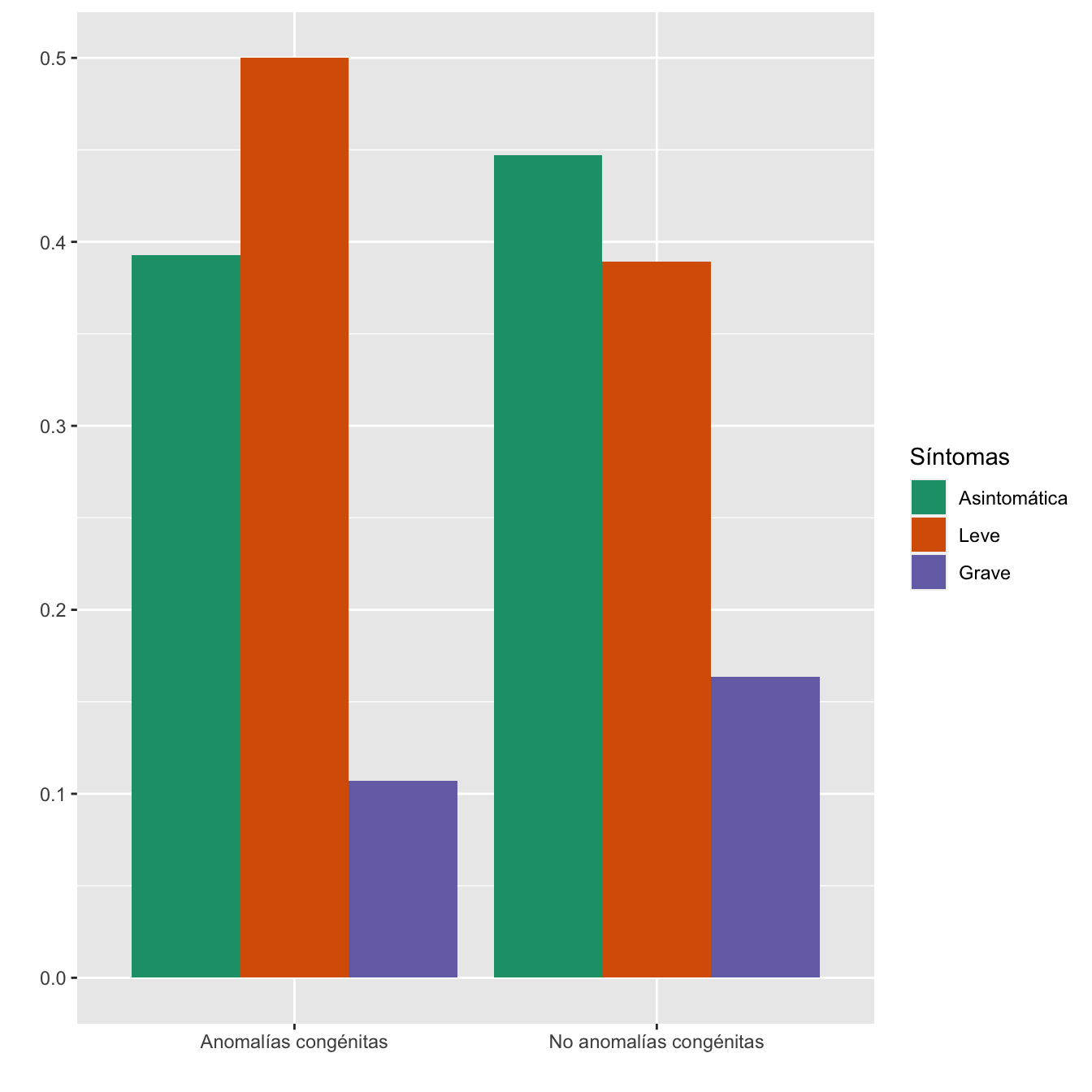
Figura 2.13:
- Potencia del test: 0.186
2.2.2 Retraso del crecimiento intrauterino
taula=table(data.frame(Casos$Defecto.del.crecimiento.fetal..en.tercer.trimestre._.CIR._.,Sint))[c(2,1) ,1:3]
Tabla.DMCasos(Casos$Defecto.del.crecimiento.fetal..en.tercer.trimestre._.CIR._.,"RCIU", "No RCIU")| Asintomáticas (N) | Asintomáticas (%) | Leves (N) | Leves (%) | Graves (N) | Graves (%) | p-valor | Tipo | |
|---|---|---|---|---|---|---|---|---|
| RCIU | 32 | 4.3 | 20 | 3.1 | 7 | 2.5 | 0.289252 | Paramétrico |
| No RCIU | 713 | 95.7 | 623 | 96.9 | 273 | 97.5 | ||
| Datos perdidos | 0 | 0 | 0 |
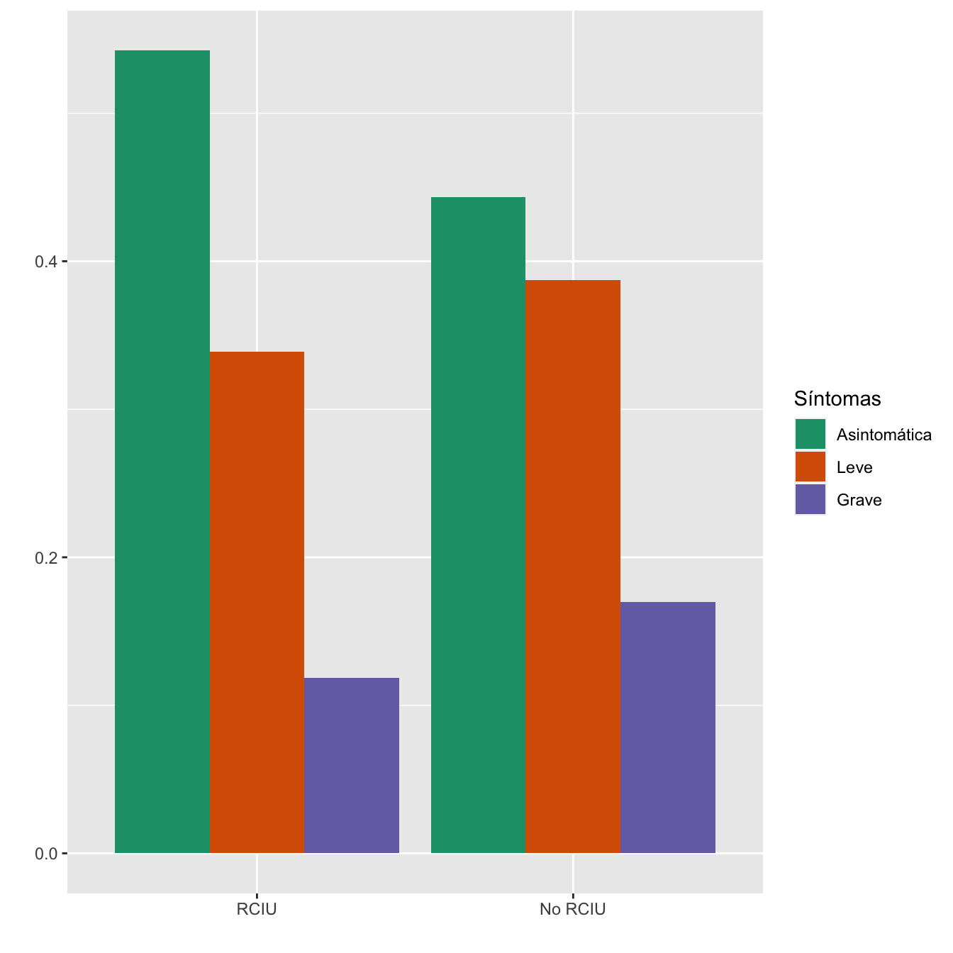
Figura 2.14:
- Potencia del test: 0.272
2.2.3 Diabetes gestacional
taula=table(data.frame(Casos$Diabetes.gestacional,Sint))[c(2,1) ,1:3]
Tabla.DMCasos(Casos$Diabetes.gestacional,"DG", "No DG")| Asintomáticas (N) | Asintomáticas (%) | Leves (N) | Leves (%) | Graves (N) | Graves (%) | p-valor | Tipo | |
|---|---|---|---|---|---|---|---|---|
| DG | 53 | 7.1 | 49 | 7.6 | 23 | 8.2 | 0.827165 | Paramétrico |
| No DG | 692 | 92.9 | 594 | 92.4 | 257 | 91.8 | ||
| Datos perdidos | 0 | 0 | 0 |
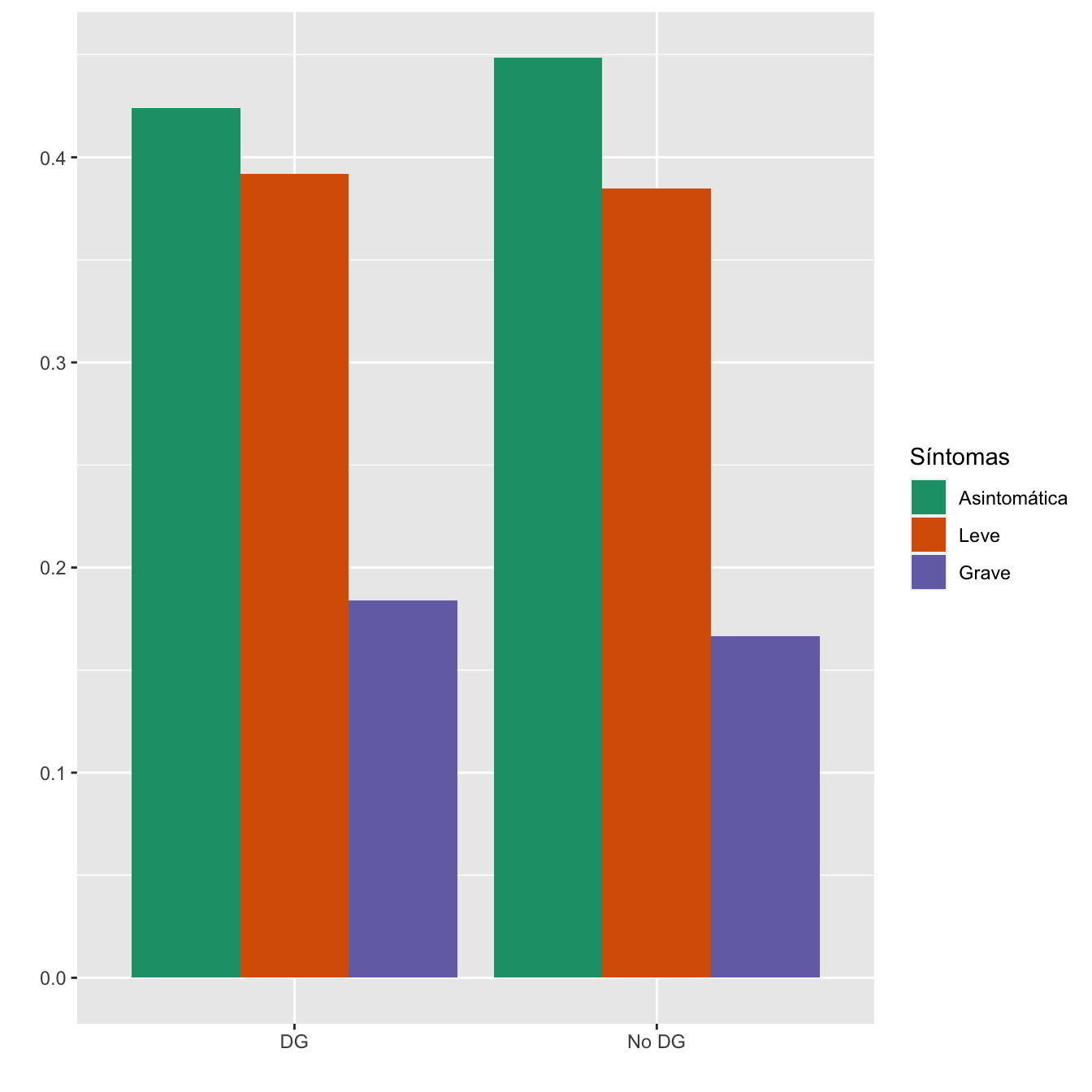
Figura 2.15:
- Potencia del test: 0.08
2.2.4 Hipertensión gestacional
taula=table(data.frame(Casos$Hipertensión.gestacional,Sint))[c(2,1) ,1:3]
Tabla.DMCasos(Casos$Hipertensión.gestacional,"HG", "No HG")| Asintomáticas (N) | Asintomáticas (%) | Leves (N) | Leves (%) | Graves (N) | Graves (%) | p-valor | Tipo | |
|---|---|---|---|---|---|---|---|---|
| HG | 20 | 2.7 | 16 | 2.5 | 6 | 2.1 | 0.883801 | Paramétrico |
| No HG | 725 | 97.3 | 627 | 97.5 | 274 | 97.9 | ||
| Datos perdidos | 0 | 0 | 0 |
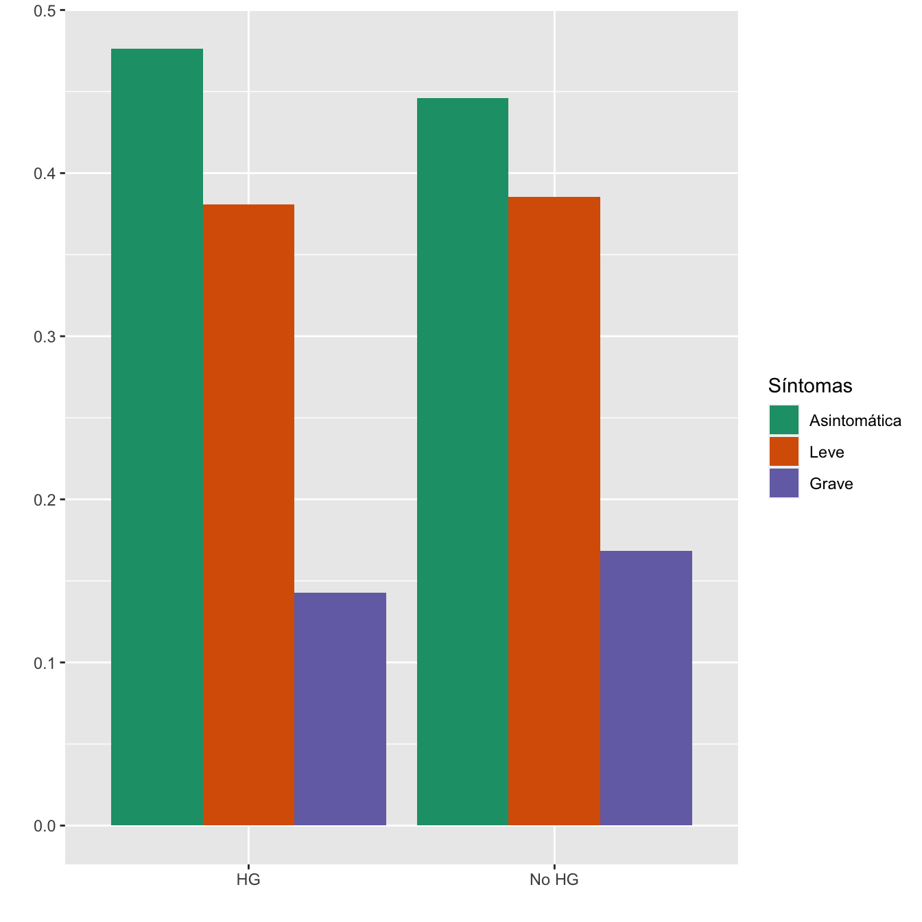
Figura 2.16:
- Potencia del test: 0.069
2.2.5 Rotura prematura de membranas
taula=table(data.frame(Casos$Bolsa.rota.anteparto,Sint))[c(2,1) ,1:3]
Tabla.DMCasos(Casos$Bolsa.rota.anteparto,"RPM", "No RPM")| Asintomáticas (N) | Asintomáticas (%) | Leves (N) | Leves (%) | Graves (N) | Graves (%) | p-valor | Tipo | |
|---|---|---|---|---|---|---|---|---|
| RPM | 103 | 13.8 | 97 | 15.1 | 35 | 12.5 | 0.56147 | Paramétrico |
| No RPM | 642 | 86.2 | 546 | 84.9 | 245 | 87.5 | ||
| Datos perdidos | 0 | 0 | 0 |
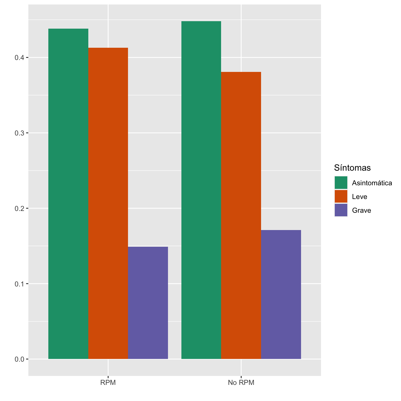
Figura 2.17:
- Potencia del test: 0.147
2.2.6 Preeclampsia
taula=table(data.frame(Casos$PREECLAMPSIA_ECLAMPSIA_TOTAL,Sint))[c(2,1) ,1:3]
Tabla.DMCasos(Casos$PREECLAMPSIA_ECLAMPSIA_TOTAL,"PE", "No PE")| Asintomáticas (N) | Asintomáticas (%) | Leves (N) | Leves (%) | Graves (N) | Graves (%) | p-valor | Tipo | |
|---|---|---|---|---|---|---|---|---|
| PE | 36 | 4.8 | 35 | 5.4 | 15 | 5.4 | 0.864429 | Paramétrico |
| No PE | 709 | 95.2 | 608 | 94.6 | 265 | 94.6 | ||
| Datos perdidos | 0 | 0 | 0 |
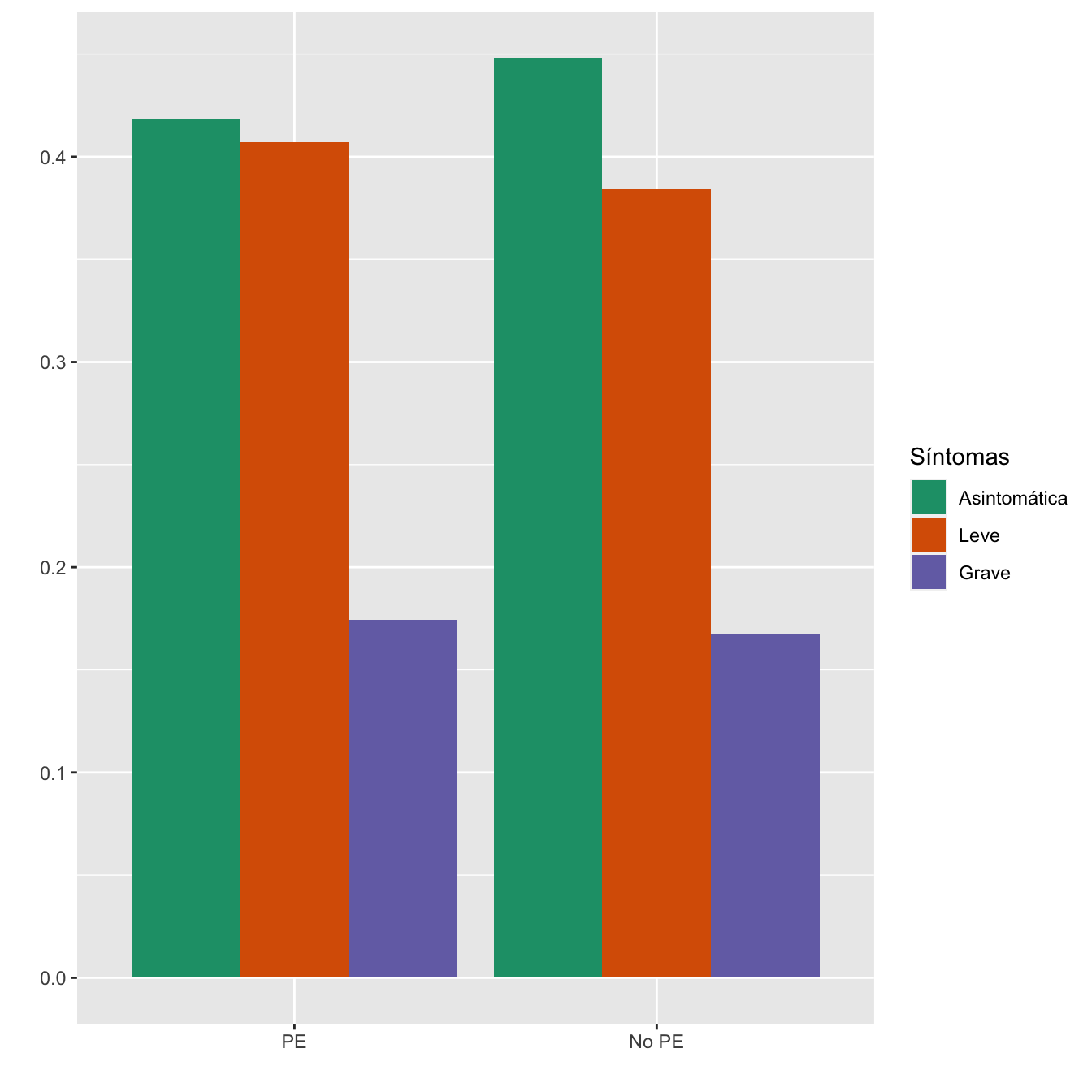
Figura 2.18:
- Potencia del test: 0.073
2.2.7 Preeclampsia con criterios de gravedad
I=Casos[Casos$PREECLAMPSIA_ECLAMPSIA_TOTAL==1,]$Preeclampsia.grave_HELLP_ECLAMPSIA
IA=Casos[Casos$PREECLAMPSIA_ECLAMPSIA_TOTAL==1 & Casos$SINTOMAS_DIAGNOSTICO=="Asintomática",]$Preeclampsia.grave_HELLP_ECLAMPSIA
IL=Casos[Casos$PREECLAMPSIA_ECLAMPSIA_TOTAL==1 & Casos$SINTOMAS_DIAGNOSTICO=="Leve",]$Preeclampsia.grave_HELLP_ECLAMPSIA
IG=Casos[Casos$PREECLAMPSIA_ECLAMPSIA_TOTAL==1 & Casos$SINTOMAS_DIAGNOSTICO=="Grave",]$Preeclampsia.grave_HELLP_ECLAMPSIA

taula=table(data.frame(I,Sint[Casos$PREECLAMPSIA_ECLAMPSIA_TOTAL==1]))
Tabla.DMCasosr(IA,IL,IG,"PE con CG", "PE sin CG")| Asintomáticas (N) | Asintomáticas (%) | Leves (N) | Leves (%) | Graves (N) | Graves (%) | p-valor | Tipo | |
|---|---|---|---|---|---|---|---|---|
| PE con CG | 9 | 25 | 13 | 37.1 | 8 | 53.3 | 0.14409 | Paramétrico |
| PE sin CG | 27 | 75 | 22 | 62.9 | 7 | 46.7 | ||
| Datos perdidos | 0 | 0 | 0 |
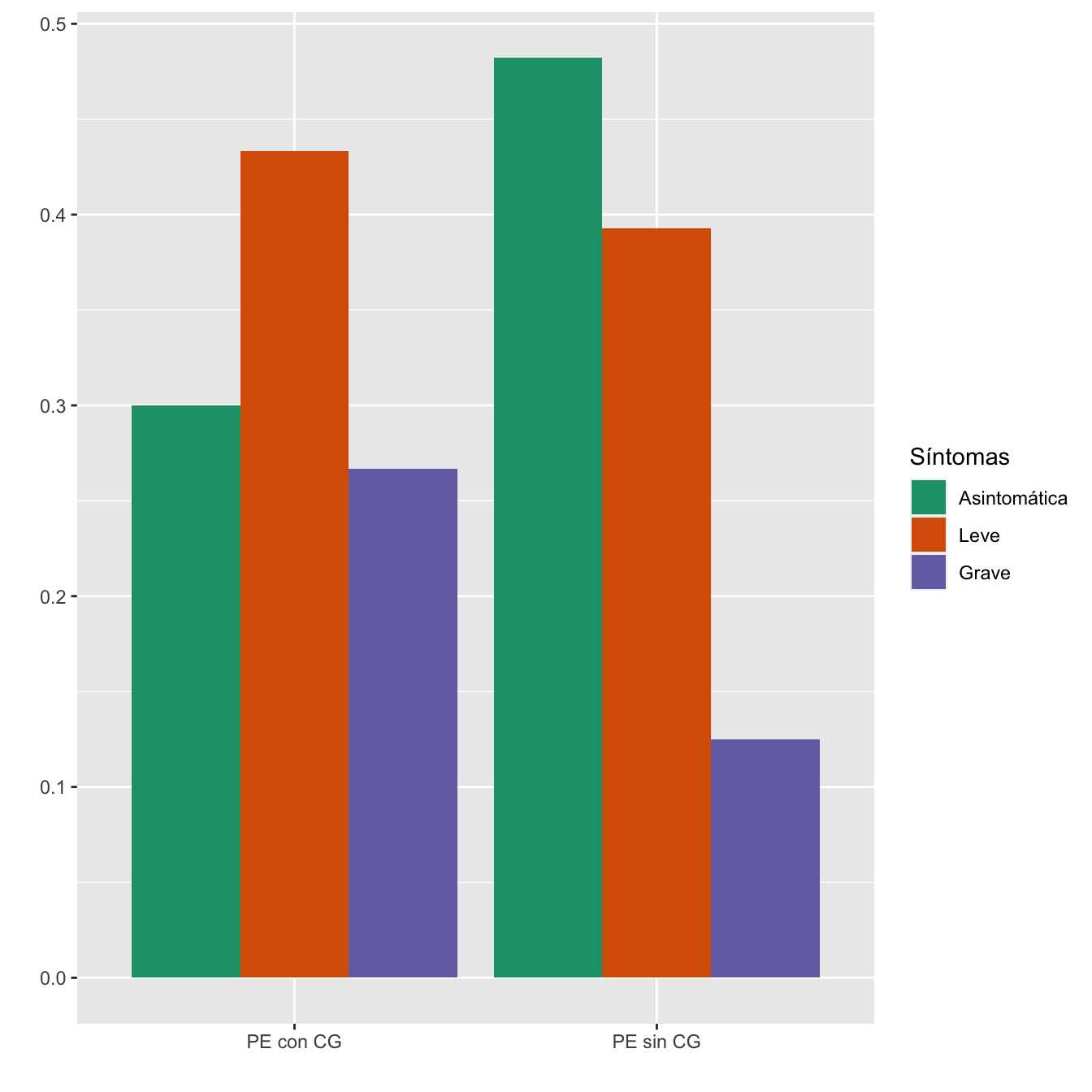
- Potencia del test: 0.404
2.2.8 Eventos hemorrágicos
taula=table(data.frame(Casos$EVENTOS_HEMORRAGICOS_TOTAL,Sint))[c(2,1) ,1:3]
Tabla.DMCasos(Casos$EVENTOS_HEMORRAGICOS_TOTAL,"Eventos hemorrágicos", "No eventos hemorrágicos")| Asintomáticas (N) | Asintomáticas (%) | Leves (N) | Leves (%) | Graves (N) | Graves (%) | p-valor | Tipo | |
|---|---|---|---|---|---|---|---|---|
| Eventos hemorrágicos | 29 | 3.9 | 39 | 6.1 | 23 | 8.2 | 0.017222 | Paramétrico |
| No eventos hemorrágicos | 716 | 96.1 | 604 | 93.9 | 257 | 91.8 | ||
| Datos perdidos | 0 | 0 | 0 |
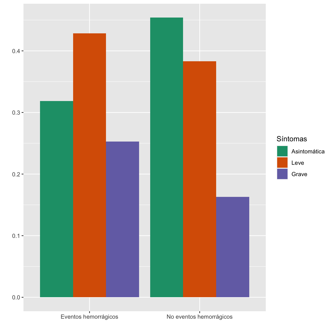
Figura 2.19:
Asociación entre los grupos de sintomatología y evento hemorrágico: test \(\chi^2\), p-valor 0.017
Test de diferencia en la tendencia de la gravedad respecto del global: p-valor 0.0269
Potencia del test: 0.725
2.2.9 Hemorragia postparto
I=Casos$Hemorragia.postparto
I.sino=I
I.sino[!is.na(I.sino)& I.sino!="No"]="Sí"
taula=table(data.frame(I.sino,Sint))[c(2,1) ,1:3]

Tabla.DMCasos(I.sino,"HPP", "No HPP")| Asintomáticas (N) | Asintomáticas (%) | Leves (N) | Leves (%) | Graves (N) | Graves (%) | p-valor | Tipo | |
|---|---|---|---|---|---|---|---|---|
| HPP | 22 | 3 | 30 | 4.7 | 21 | 7.9 | 0.003746 | Paramétrico |
| No HPP | 710 | 97 | 607 | 95.3 | 244 | 92.1 | ||
| Datos perdidos | 13 | 6 | 15 |
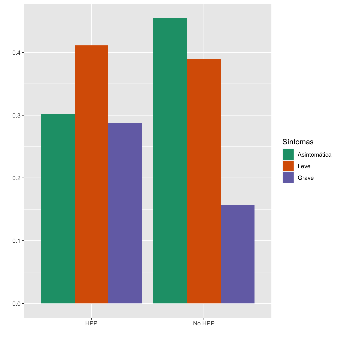
Figura 2.20:
- Potencia del test: 0.858
I=ordered(I,levels=names(table(I))[c(2,3,1,4)])
Tabla.DMCasosm(I,c("Tto. médico",
  "Tto. Qx. conservador" , "Histerectomía",
"No") ,r=6)| Asintomáticas (N) | Asintomáticas (%) | Leves (N) | Leves (%) | Graves (N) | Graves (%) | p-valor | Tipo | |
|---|---|---|---|---|---|---|---|---|
| Tto. médico | 20 | 2.7 | 23 | 3.6 | 16 | 6.0 | 0.188670 | Paramétrico |
| Tto. Qx. conservador | 2 | 0.3 | 4 | 0.6 | 3 | 1.1 | 1.000000 | Montecarlo |
| Histerectomía | 0 | 0.0 | 3 | 0.5 | 2 | 0.8 | 0.300770 | Montecarlo |
| No | 710 | 97.0 | 607 | 95.3 | 244 | 92.1 | 0.014985 | Paramétrico |
| Datos perdidos | 13 | 6 | 15 |
DF=data.frame(Factor=I,Síntomas=Sint)
taula=table(DF)

Síntomas=ordered(rep(c("Asintomática", "Leve", "Grave"), each=4),levels=c("Asintomática", "Leve", "Grave"))
Grupo=ordered(rep(c("Tto. médico",
  "Tto. Qx. conservador" , "Histerectomía" ,
"No") , 3),levels=c("Tto. médico",
  "Tto. Qx. conservador" , "Histerectomía",
"No"))
valor=as.vector(prop.table(taula, margin=1))
data <- data.frame(Grupo,Síntomas,valor)

ggplot(data, aes(fill=Síntomas, y=valor, x=Grupo)) +
  geom_bar(position="dodge", stat="identity")+
  ylab("")+
  xlab("")+
scale_fill_brewer(palette = "Dark2") 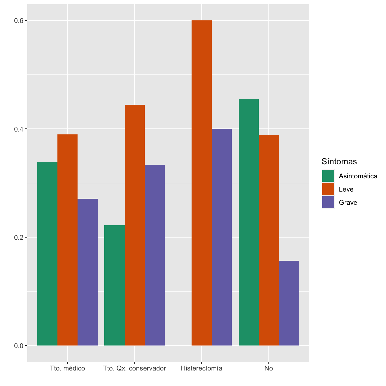
Figura 2.21:
Asociación entre los grupos de sintomatología y el tipo de hemorragia postparto: test \(\chi^2\) de Montecarlo, p-valor 0.608
Potencia del test: 0.232
2.2.10 Eventos trombóticos
taula=table(data.frame(Casos$EVENTOS_TROMBO_TOTALES,Sint))[c(2,1) ,1:3]
Tabla.DMCasos(Casos$EVENTOS_TROMBO_TOTALES,"Eventos trombóticos", "No eventos trombóticos")| Asintomáticas (N) | Asintomáticas (%) | Leves (N) | Leves (%) | Graves (N) | Graves (%) | p-valor | Tipo | |
|---|---|---|---|---|---|---|---|---|
| Eventos trombóticos | 1 | 0.1 | 0 | 0 | 11 | 3.9 | 1e-04 | Montecarlo |
| No eventos trombóticos | 744 | 99.9 | 643 | 100 | 269 | 96.1 | ||
| Datos perdidos | 0 | 0 | 0 |
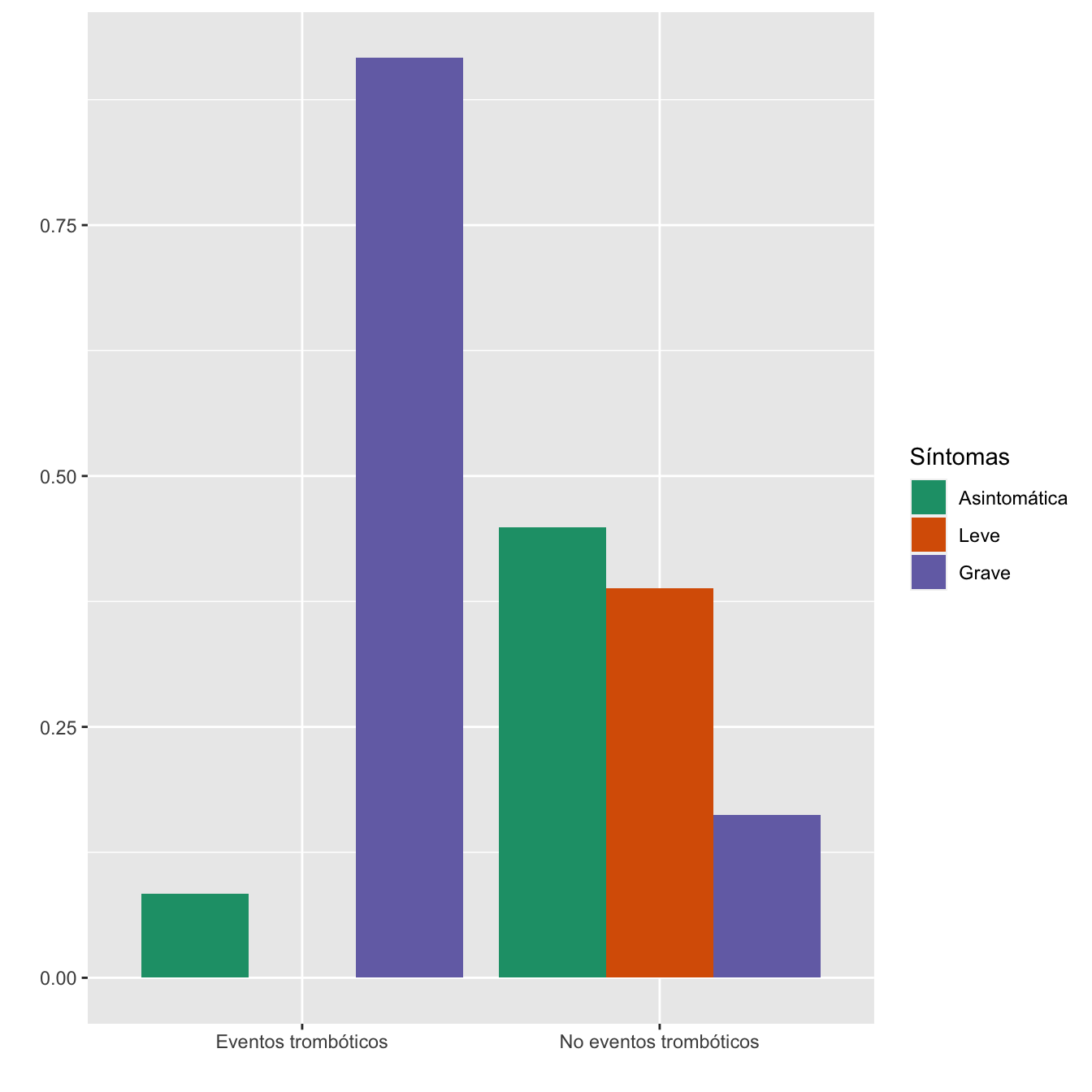
Figura 2.22:
- Potencia del test: 1
2.2.11 UCI materna (Sí-No)
| Asintomáticas (N) | Asintomáticas (%) | Leves (N) | Leves (%) | Graves (N) | Graves (%) | p-valor | Tipo | |
|---|---|---|---|---|---|---|---|---|
| UCI | 3 | 0.4 | 7 | 1.1 | 27 | 9.6 | 0 | Paramétrico |
| No UCI | 742 | 99.6 | 636 | 98.9 | 253 | 90.4 | ||
| Datos perdidos | 0 | 0 | 0 |
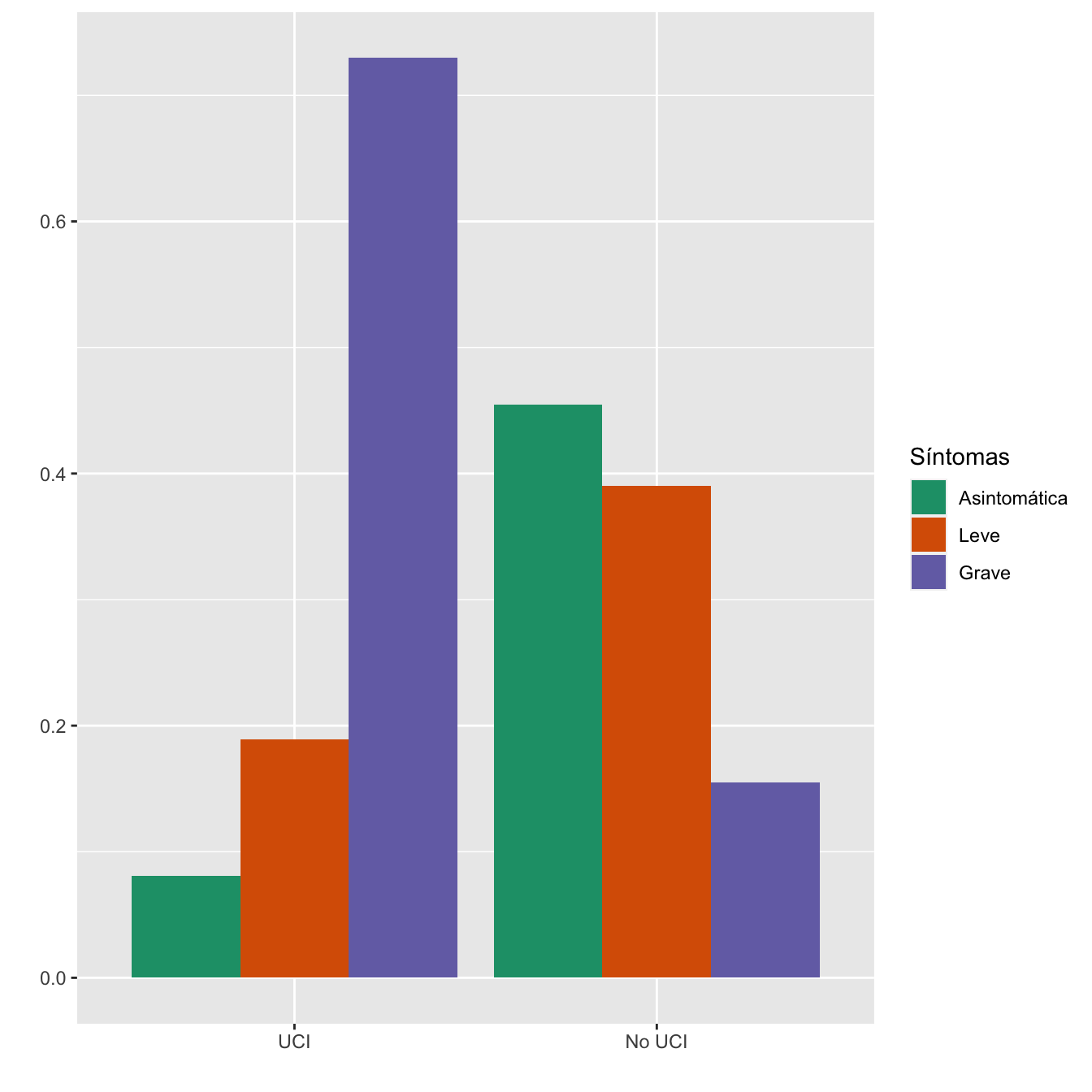
Figura 2.23:
- Potencia del test: 1
2.2.12 UCI materna (antes-después)
I=Casos$UCI_ANTES.DESPUES.DEL.PARTO[Casos$UCI==1]
IA=Casos[Casos$UCI==1 & Casos$SINTOMAS_DIAGNOSTICO=="Asintomática",]$UCI_ANTES.DESPUES.DEL.PARTO
IA=factor(IA,levels=c("ANTES DEL PARTO","DESPUES DEL PARTO"))
IL=Casos[Casos$UCI==1 & Casos$SINTOMAS_DIAGNOSTICO=="Leve",]$UCI_ANTES.DESPUES.DEL.PARTO
IG=Casos[Casos$UCI==1 & Casos$SINTOMAS_DIAGNOSTICO=="Grave",]$UCI_ANTES.DESPUES.DEL.PARTO

taula=table(data.frame(I,Sint[Casos$UCI==1]))
Tabla.DMCasosr(IA,IL,IG,"UCI antes del parto", "UCI después del parto")| Asintomáticas (N) | Asintomáticas (%) | Leves (N) | Leves (%) | Graves (N) | Graves (%) | p-valor | Tipo | |
|---|---|---|---|---|---|---|---|---|
| UCI antes del parto | 3 | 100 | 5 | 71.4 | 19 | 70.4 | 0.70493 | Montecarlo |
| UCI después del parto | 0 | 0 | 2 | 28.6 | 8 | 29.6 | ||
| Datos perdidos | 0 | 0 | 0 |
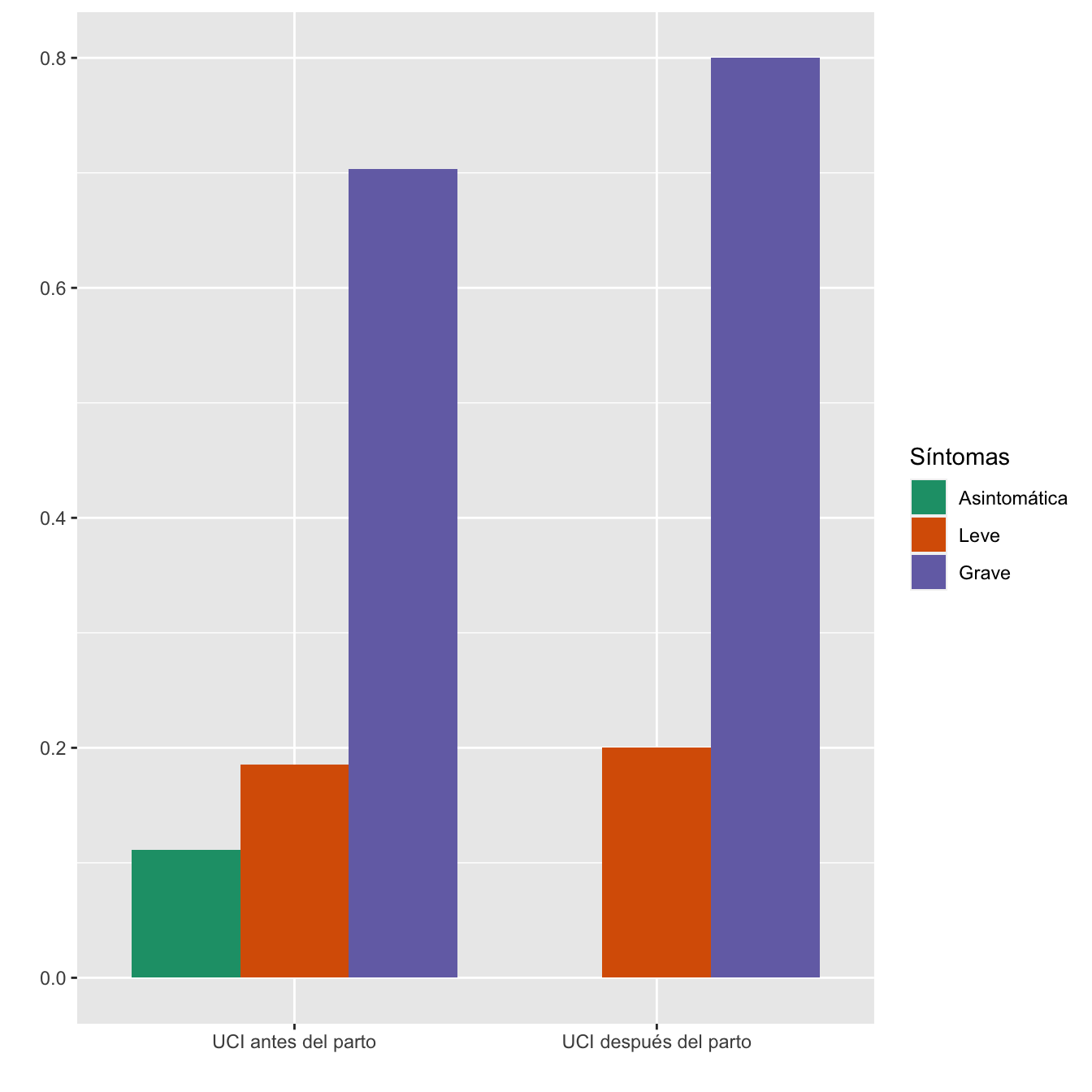
- Potencia del test: 0.152
2.2.13 Prematuridad
taula=table(data.frame(Casos$PREMATURO,Sint))[c(2,1) ,1:3]
Tabla.DMCasos(Casos$PREMATURO,"Prematuro", "A término")| Asintomáticas (N) | Asintomáticas (%) | Leves (N) | Leves (%) | Graves (N) | Graves (%) | p-valor | Tipo | |
|---|---|---|---|---|---|---|---|---|
| Prematuro | 53 | 7.1 | 63 | 9.8 | 53 | 18.9 | 0 | Paramétrico |
| A término | 692 | 92.9 | 580 | 90.2 | 227 | 81.1 | ||
| Datos perdidos | 0 | 0 | 0 |
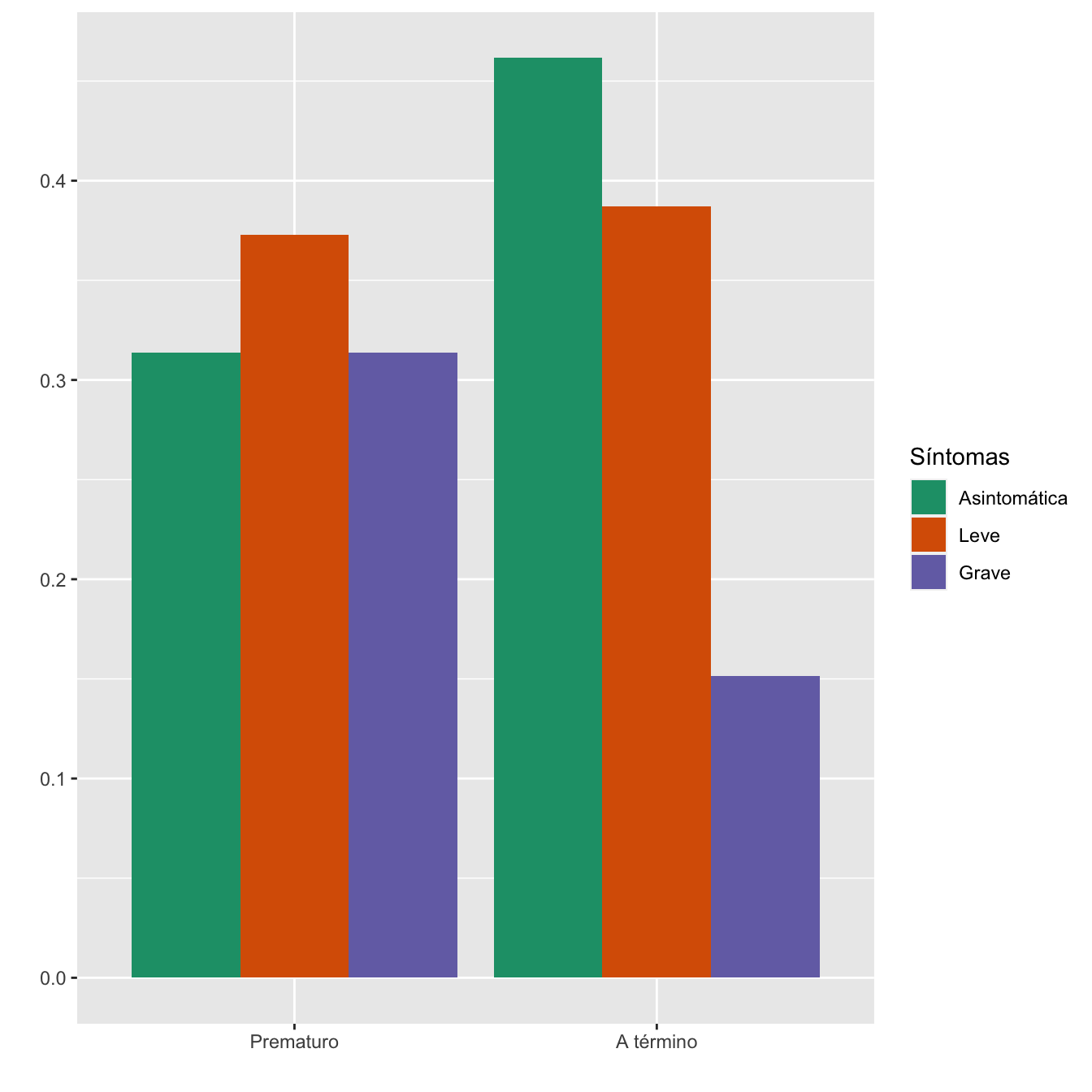
Figura 2.24:
- Potencia del test: 0.999
2.2.14 Inicio de parto
I=Casos$Inicio.de.parto
I=factor(I,levels=c("Espontáneo", "Inducido", "Cesárea"),ordered=TRUE)
DF=data.frame(Factor=I,Síntomas=Sint)
taula=table(DF)
Tabla.DMCasosm(I,c("Espontáneo", "Inducido","Cesárea programada"))| Asintomáticas (N) | Asintomáticas (%) | Leves (N) | Leves (%) | Graves (N) | Graves (%) | p-valor | Tipo | |
|---|---|---|---|---|---|---|---|---|
| Espontáneo | 423 | 56.8 | 332 | 51.7 | 116 | 41.6 | 0.000232 | Paramétrico |
| Inducido | 273 | 36.6 | 246 | 38.3 | 109 | 39.1 | 1.000000 | Paramétrico |
| Cesárea programada | 49 | 6.6 | 64 | 10.0 | 54 | 19.4 | 0.000000 | Paramétrico |
| Datos perdidos | 0 | 1 | 1 |
Síntomas=ordered(rep(c("Asintomática", "Leve", "Grave"), each=3),levels=c("Asintomática", "Leve", "Grave"))
Grupo=ordered(rep(rownames(EEExt)[1:3] , 3),levels=rownames(EEExt)[1:3])
valor=as.vector(prop.table(taula, margin=1))
data <- data.frame(Grupo,Síntomas,valor)

ggplot(data, aes(fill=Síntomas, y=valor, x=Grupo)) +
  geom_bar(position="dodge", stat="identity")+
  ylab("")+
  xlab("Inicio de parto")+
scale_fill_brewer(palette = "Dark2") 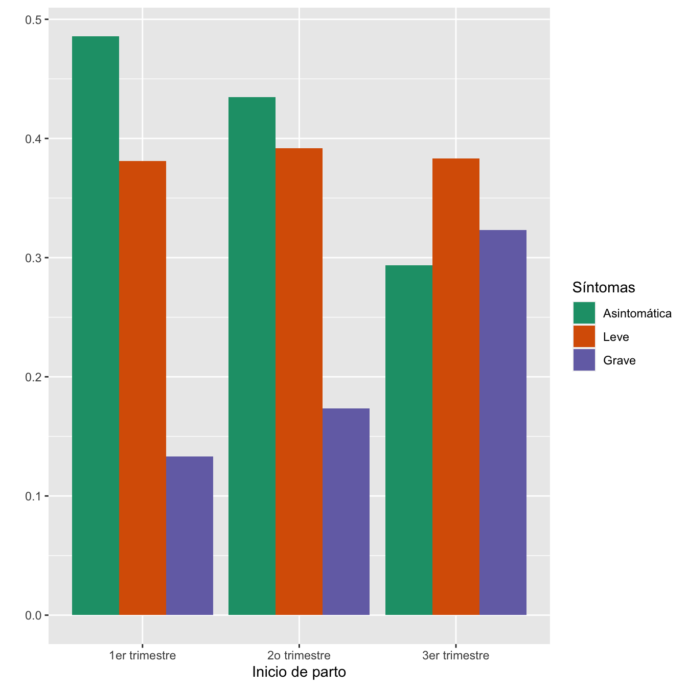
Figura 2.25:
- Asociación entre los grupos de sintomatología y el inicio de parto: test \(\chi^2\), p-valor \(10^{-8}\)
2.2.15 Tipo de parto
I.In=Casos$Inicio.de.parto
I.In[I.In=="Cesárea"]="Cesárea programada"
I=Casos$Tipo.de.parto
I[I.In=="Cesárea programada"]="Cesárea programada"
I[I=="Cesárea"]="Cesárea urgente"

I=factor(I,levels=c("Eutocico", "Instrumental", "Cesárea programada", "Cesárea urgente"),ordered=TRUE)
DF=data.frame(Factor=I,Síntomas=Sint)
taula=table(DF)
Tabla.DMCasosm(I,c("Eutócico", "Instrumental", "Cesárea programada", "Cesárea urgente"))| Asintomáticas (N) | Asintomáticas (%) | Leves (N) | Leves (%) | Graves (N) | Graves (%) | p-valor | Tipo | |
|---|---|---|---|---|---|---|---|---|
| Eutócico | 488 | 65.5 | 412 | 64.1 | 155 | 55.4 | 0.037871 | Paramétrico |
| Instrumental | 85 | 11.4 | 71 | 11.0 | 21 | 7.5 | 0.700856 | Paramétrico |
| Cesárea programada | 49 | 6.6 | 64 | 10.0 | 54 | 19.3 | 0.000000 | Paramétrico |
| Cesárea urgente | 123 | 16.5 | 96 | 14.9 | 50 | 17.9 | 1.000000 | Paramétrico |
| Datos perdidos | 0 | 0 | 0 |
Síntomas=ordered(rep(c("Asintomática", "Leve", "Grave"), each=4),levels=c("Asintomática", "Leve", "Grave"))
Grupo=ordered(rep(c("Eutócico", "Instrumental", "Cesárea programada", "Cesárea urgente") , 3),levels=c("Eutócico", "Instrumental", "Cesárea programada", "Cesárea urgente"))
valor=as.vector(prop.table(taula, margin=1))
data <- data.frame(Grupo,Síntomas,valor)

ggplot(data, aes(fill=Síntomas, y=valor, x=Grupo)) +
  geom_bar(position="dodge", stat="identity")+
  ylab("")+
  xlab("Tipo de parto")+
scale_fill_brewer(palette = "Dark2") 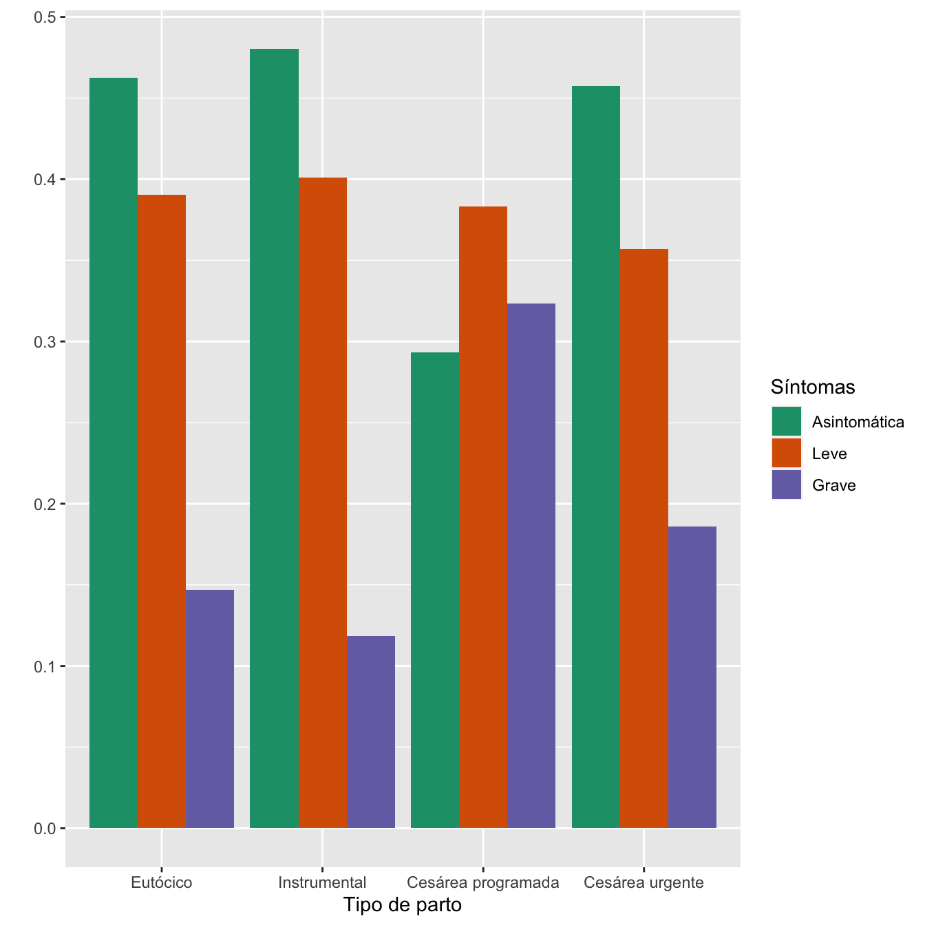
Figura 2.26:
Asociación entre los grupos de sintomatología y tipos de parto: test \(\chi^2\), p-valor \(4\times 10^{-7}\)
Asociación entre los grupos de sintomatología y tipos de parto diferentes de la cesárea programada: test \(\chi^2\), p-valor 0.354
2.2.16 APGAR
I=c(Casos$APGAR.5...126,CasosGM$APGAR.5...150)
I[I==19]=NA
I=cut(I,breaks=c(-1,7,20),labels=c("0-7","8-10"))
I=ordered(I,levels=c("8-10","0-7"))
SintN=c(Casos$SINTOMAS_DIAGNOSTICO,CasosGM$SINTOMAS_DIAGNOSTICO)

taula=table(data.frame(I,SintN))[c(2,1) ,1:3]
Tabla.DMCasos(I,"Apgar.5≤7","Apgar.5≥8")| Asintomáticas (N) | Asintomáticas (%) | Leves (N) | Leves (%) | Graves (N) | Graves (%) | p-valor | Tipo | |
|---|---|---|---|---|---|---|---|---|
| Apgar.5≤7 | 19 | 2.6 | 20 | 3 | 11 | 4 | 0.502207 | Paramétrico |
| Apgar.5≥8 | 723 | 97.4 | 637 | 97 | 267 | 96 | ||
| Datos perdidos | 12 | 7 | 3 |
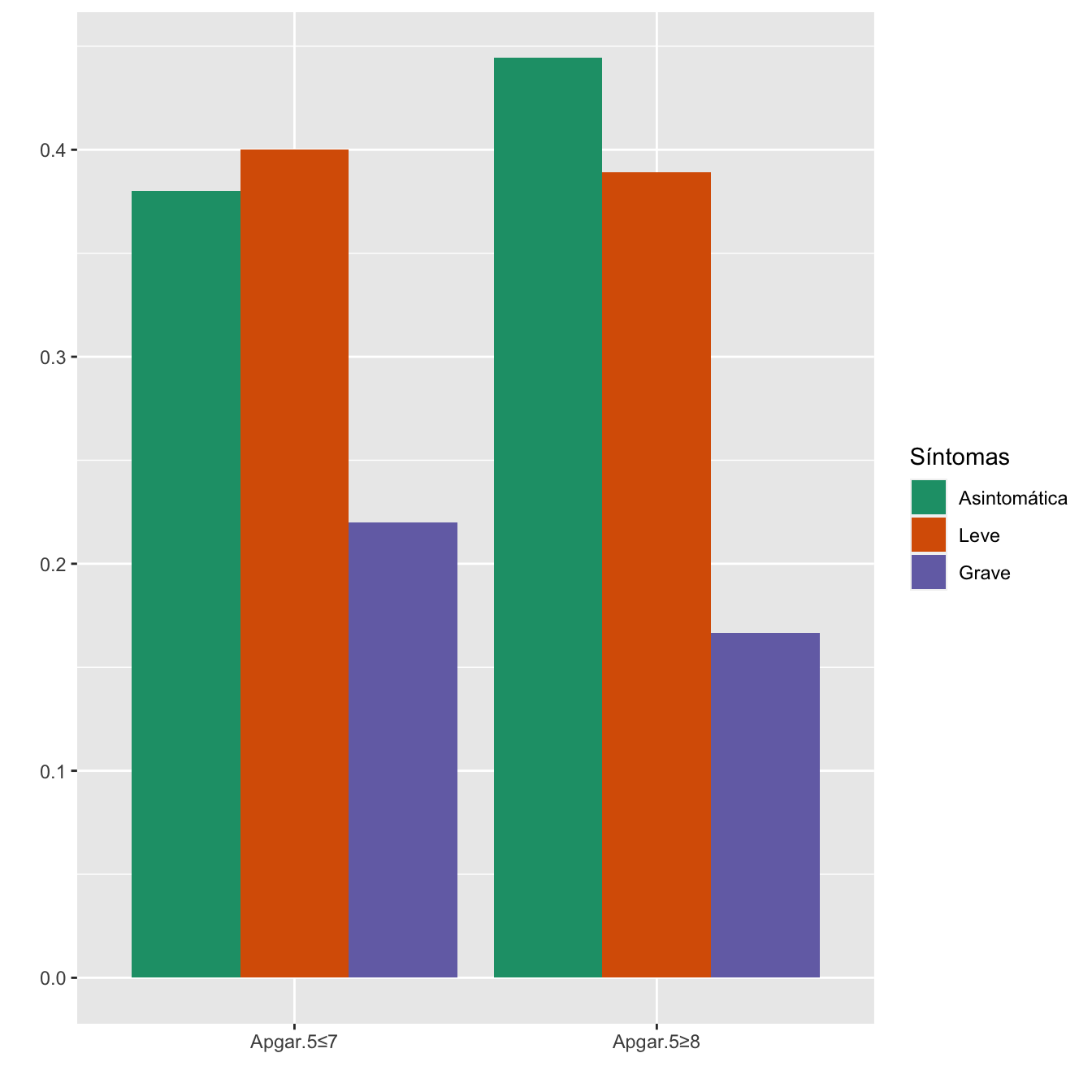
- Potencia del test: 0.159
2.2.17 Sintomatología vs UCI neonato
I=c(Casos[Casos$Feto.muerto.intraútero=="No",]$Ingreso.en.UCIN,CasosGM[CasosGM$Feto.vivo=="Sí",]$Ingreso.en.UCI)

IA=c(Casos[Casos$SINTOMAS_DIAGNOSTICO=="Asintomática"&Casos$Feto.muerto.intraútero=="No",]$Ingreso.en.UCIN,CasosGM[CasosGM$SINTOMAS_DIAGNOSTICO=="Asintomática" & CasosGM$Feto.vivo=="Sí",]$Ingreso.en.UCI)

IL=c(Casos[Casos$SINTOMAS_DIAGNOSTICO=="Leve"&Casos$Feto.muerto.intraútero=="No",]$Ingreso.en.UCIN,CasosGM[CasosGM$SINTOMAS_DIAGNOSTICO=="Leve" & CasosGM$Feto.vivo=="Sí",]$Ingreso.en.UCI)

IG=c(Casos[Casos$SINTOMAS_DIAGNOSTICO=="Grave"&Casos$Feto.muerto.intraútero=="No",]$Ingreso.en.UCIN,CasosGM[CasosGM$SINTOMAS_DIAGNOSTICO=="Grave" & CasosGM$Feto.vivo=="Sí",]$Ingreso.en.UCI)

SintN=c(Casos[Casos$Feto.muerto.intraútero=="No",]$SINTOMAS_DIAGNOSTICO,CasosGM[CasosGM$Feto.vivo=="Sí",]$SINTOMAS_DIAGNOSTICO)

taula=table(data.frame(I,SintN))[c(2,1) ,1:3]
Tabla.DMCasosr(IA,IL,IG,"UCIN", "No UCIN")| Asintomáticas (N) | Asintomáticas (%) | Leves (N) | Leves (%) | Graves (N) | Graves (%) | p-valor | Tipo | |
|---|---|---|---|---|---|---|---|---|
| UCIN | 52 | 7.1 | 55 | 8.6 | 50 | 17.8 | 1e-06 | Paramétrico |
| No UCIN | 682 | 92.9 | 588 | 91.4 | 231 | 82.2 | ||
| Datos perdidos | 11 | 8 | 3 |
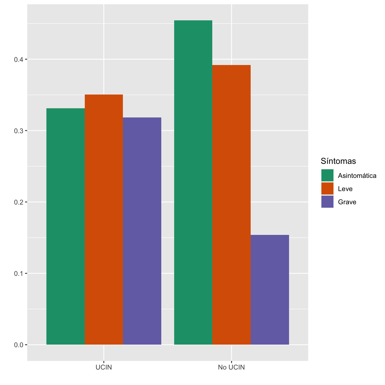
- Potencia del test: 0.999
2.2.18 Sintomatología vs Fetos muertos anteparto
I1=Casos$Feto.muerto.intraútero
I1[I1=="Sí"]="Muerto"
I1[I1=="No"]="Vivo"
I1=ordered(I1,levels=c("Vivo","Muerto"))
I1A=I1[Casos$SINTOMAS_DIAGNOSTICO=="Asintomática"]
I1L=I1[Casos$SINTOMAS_DIAGNOSTICO=="Leve"]
I1G=I1[Casos$SINTOMAS_DIAGNOSTICO=="Grave"]

I2=CasosGM$Feto.vivo
I2[I2=="Sí"]="Vivo"
I2[I2=="No"]="Muerto"
I2=ordered(I2,levels=c("Vivo","Muerto"))
I2A=I2[CasosGM$SINTOMAS_DIAGNOSTICO=="Asintomática"]
I2L=I2[CasosGM$SINTOMAS_DIAGNOSTICO=="Leve"]
I2G=I2[CasosGM$SINTOMAS_DIAGNOSTICO=="Grave"]

IA=c(I1A,I2A)
IL=c(I1L,I2L)
IG=c(I1G,I2G)


I=c(I1,I2)
SintN1=Casos$SINTOMAS_DIAGNOSTICO
SintN2=CasosGM$SINTOMAS_DIAGNOSTICO
SintN=c(SintN1,SintN2)

taula=table(data.frame(I,SintN))[c(2,1) ,1:3]
Tabla.DMCasosr(IA,IL,IG,"Feto muerto anteparto", "Feto vivo")| Asintomáticas (N) | Asintomáticas (%) | Leves (N) | Leves (%) | Graves (N) | Graves (%) | p-valor | Tipo | |
|---|---|---|---|---|---|---|---|---|
| Feto muerto anteparto | 8 | 1.1 | 9 | 1.4 | 2 | 0.7 | 0.644936 | Montecarlo |
| Feto vivo | 745 | 98.9 | 650 | 98.6 | 284 | 99.3 | ||
| Datos perdidos | 0 | 1 | 0 |
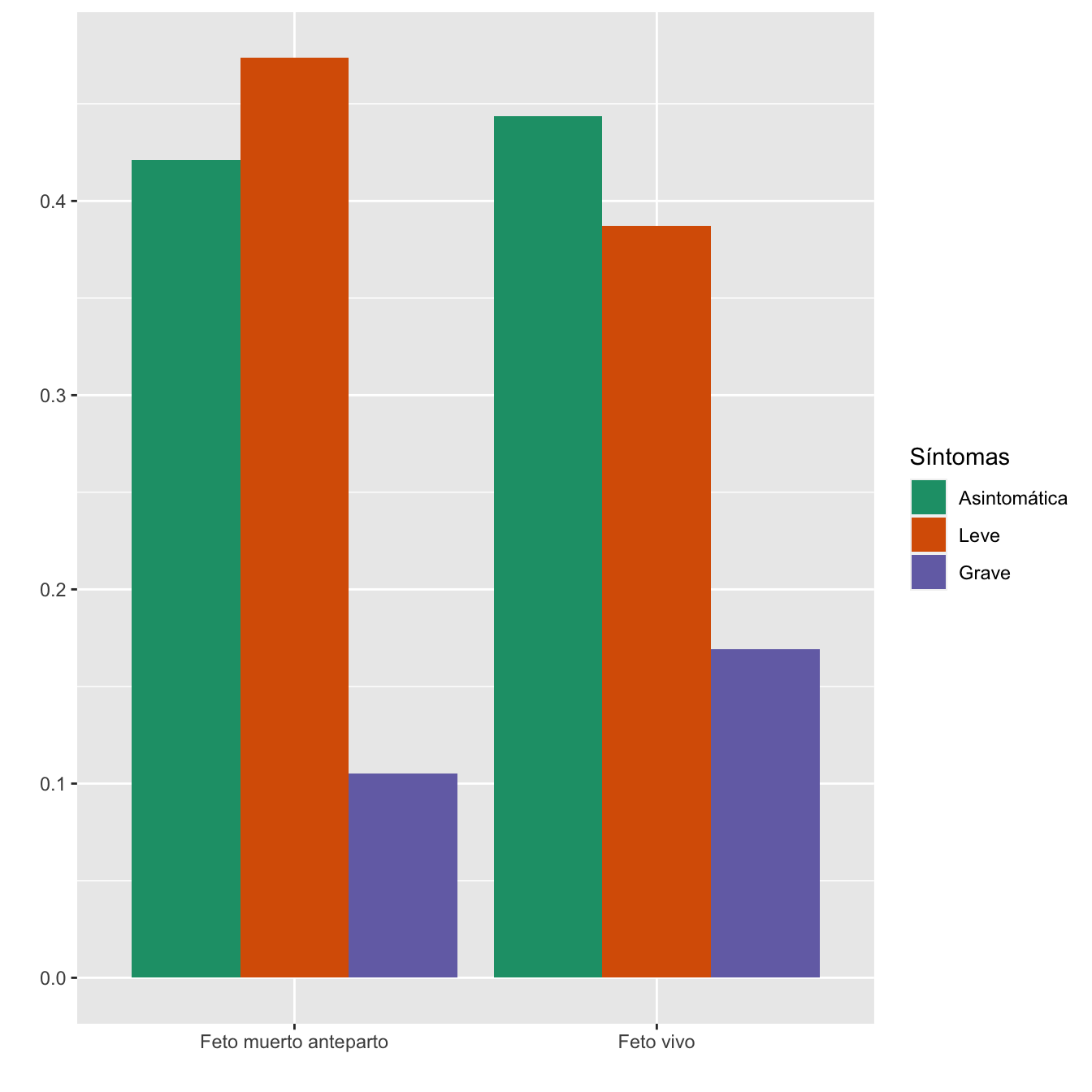
- Potencia del test: 0.119
2.2.19 Edades gestacionales
I=Casos$EG_TOTAL_PARTO
Síntomas=ordered(Sint,levels=c("Asintomática" ,"Leve",      "Grave"  ))
data =data.frame(
  Síntomas,
  Edades=I
)

data %>%
  ggplot( aes(x=Síntomas, y=Edades, fill=Síntomas)) +
    geom_violin(width=1) +
    geom_boxplot(width=0.1, color="black", alpha=0.2,outlier.fill="black",
               outlier.size=1) +
    theme(
      legend.position="none",
      plot.title = element_text(size=11)
    ) +
    xlab("")+
   ylab("Edades gestacionales (semanas)")+
scale_fill_brewer(palette = "Dark2") 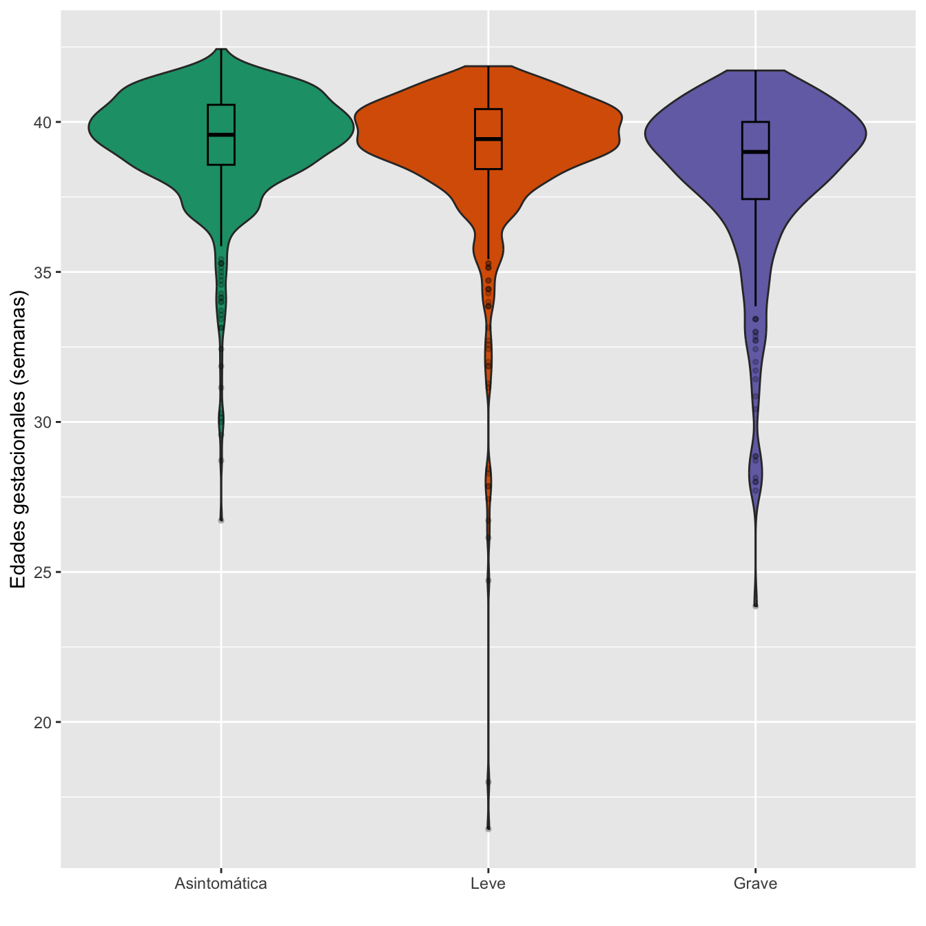
Figura 2.27:
Dades=rbind(c(round(min(I[data$Síntomas=="Asintomática"],na.rm=TRUE),1),round(max(I[data$Síntomas=="Asintomática"],na.rm=TRUE),1), round(mean(I[data$Síntomas=="Asintomática"],na.rm=TRUE),1),
              round(median(I[data$Síntomas=="Asintomática"],na.rm=TRUE),1),
              round(quantile(I[data$Síntomas=="Asintomática"],c(0.25,0.75),na.rm=TRUE),1),
              round(sd(I[data$Síntomas=="Asintomática"],na.rm=TRUE),1)),
   c(round(min(I[data$Síntomas=="Leve"],na.rm=TRUE),1),round(max(I[data$Síntomas=="Leve"],na.rm=TRUE),1), round(mean(I[data$Síntomas=="Leve"],na.rm=TRUE),1),
       round(median(I[data$Síntomas=="Leve"],na.rm=TRUE),1),
              round(quantile(I[data$Síntomas=="Leve"],c(0.25,0.75),na.rm=TRUE),1),round(sd(I[data$Síntomas=="Leve"],na.rm=TRUE),1)),
  c(round(min(I[data$Síntomas=="Grave"],na.rm=TRUE),1),round(max(I[data$Síntomas=="Grave"],na.rm=TRUE),1), round(mean(I[data$Síntomas=="Grave"],na.rm=TRUE),1),round(median(I[data$Síntomas=="Grave"],na.rm=TRUE),1),
              round(quantile(I[data$Síntomas=="Grave"],c(0.25,0.75),na.rm=TRUE),1),round(sd(I[data$Síntomas=="Grave"],na.rm=TRUE),1))          )

colnames(Dades)=c("Edad gest. mínima","Edad gest.  máxima","Edad gest.  media",
                  "Edad gest. mediana", "1er cuartil", "3er cuartil","Desv. típica")
rownames(Dades)=c("Asintomática" ,"Leve",      "Grave"  )

Dades %>%
  kbl() %>%
  kable_styling() %>%
scroll_box(width="100%", box_css="border: 0px;")| Edad gest. mínima | Edad gest. máxima | Edad gest. media | Edad gest. mediana | 1er cuartil | 3er cuartil | Desv. típica | |
|---|---|---|---|---|---|---|---|
| Asintomática | 26.7 | 42.4 | 39.3 | 39.6 | 38.6 | 40.6 | 1.9 |
| Leve | 16.4 | 41.9 | 39.0 | 39.4 | 38.4 | 40.4 | 2.5 |
| Grave | 23.9 | 41.7 | 38.3 | 39.0 | 37.4 | 40.0 | 2.8 |
Ajuste de las edades gestacionales de cada nivel a distribuciones normales: test de Shapiro-Wilks, p-valores \(9\times 10^{-26}\), \(10^{-32}\), \(2\times 10^{-17}\), respectivamente
Homocedasticidad: Test de Fligner-Killeen, p-valor \(10^{-5}\)
Edades gestacionales medias: test de Kruskal-Wallis, p-valor \(2\times 10^{-7}\)
Contrastes posteriores de edades gestacionales medias por parejas: tests de Mann-Whitney,p-valores ajustados por Bonferroni:
- Asintomática vs Leve: 0.188
- Asintomática vs Grave: \(9\times 10^{-8}\)
- Leve vs Grave: \(10^{-4}\)
2.2.20 Pesos hijos infectadas
SintN=c(Casos[Casos$Feto.muerto.intraútero=="No",]$SINTOMAS_DIAGNOSTICO,CasosGM[CasosGM$Feto.vivo=="Sí",]$SINTOMAS_DIAGNOSTICO)
Síntomas=SintN[!is.na(SintN)]

I=c(Casos[Casos$Feto.muerto.intraútero=="No",]$Peso._gramos_...125,CasosGM[CasosGM$Feto.vivo=="Sí",]$Peso._gramos_...148)
I=I[!is.na(SintN)]

data =data.frame(
  Síntomas,
  Pesos=I
)

data %>%
  ggplot( aes(x=Síntomas, y=Pesos, fill=Síntomas)) +
    geom_violin(width=1) +
    geom_boxplot(width=0.1, color="black", alpha=0.2,outlier.fill="black",
               outlier.size=1) +
    theme(
      legend.position="none",
      plot.title = element_text(size=11)
    ) +
    xlab("")+
   ylab("Pesos (gramos)")+
scale_fill_brewer(palette = "Dark2") 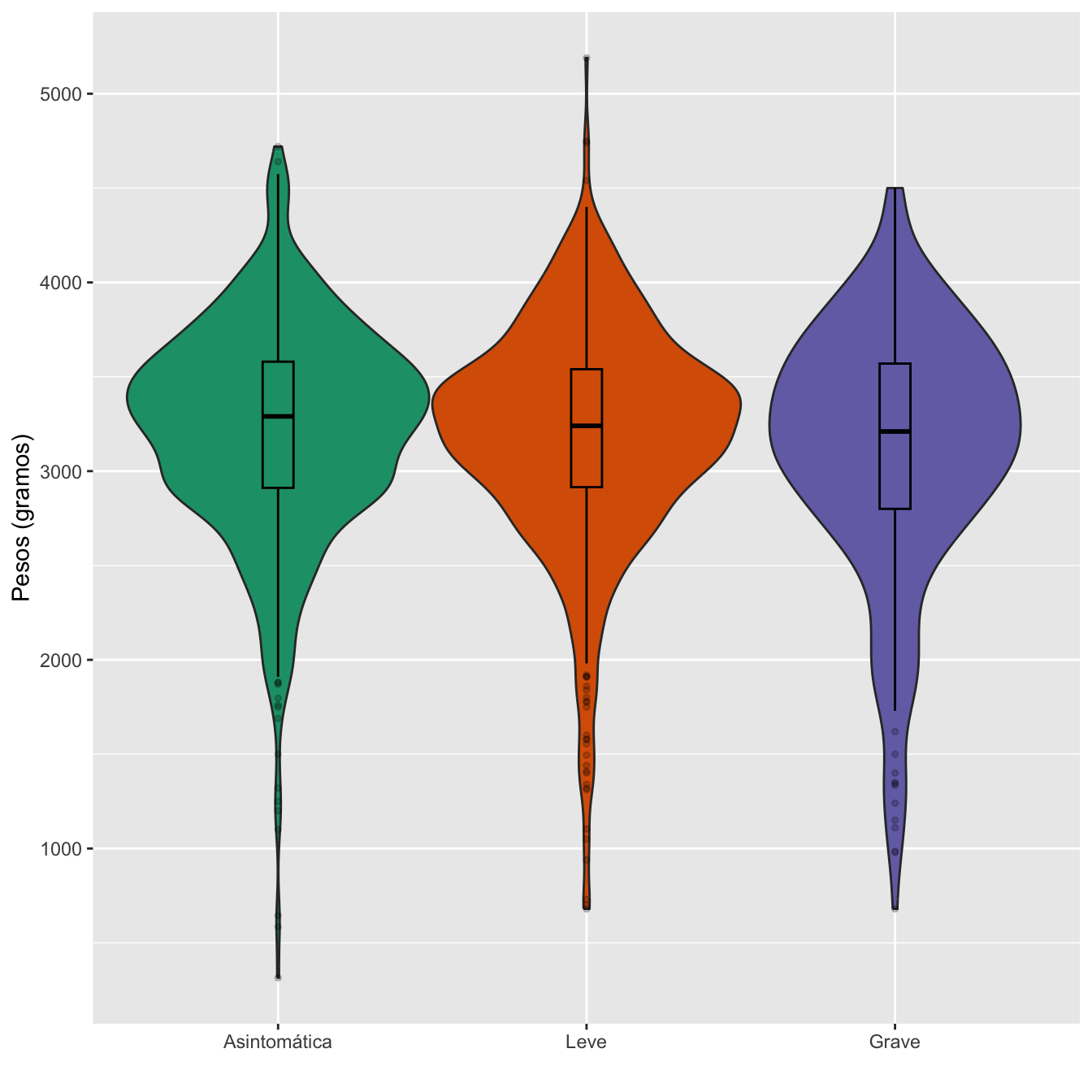
Figura 2.28:
Dades=rbind(c(round(min(I[data$Síntomas=="Asintomática"],na.rm=TRUE),1),round(max(I[data$Síntomas=="Asintomática"],na.rm=TRUE),1), round(mean(I[data$Síntomas=="Asintomática"],na.rm=TRUE),1),
              round(median(I[data$Síntomas=="Asintomática"],na.rm=TRUE),1),
              round(quantile(I[data$Síntomas=="Asintomática"],c(0.25,0.75),na.rm=TRUE),1),
              round(sd(I[data$Síntomas=="Asintomática"],na.rm=TRUE),1)),
   c(round(min(I[data$Síntomas=="Leve"],na.rm=TRUE),1),round(max(I[data$Síntomas=="Leve"],na.rm=TRUE),1), round(mean(I[data$Síntomas=="Leve"],na.rm=TRUE),1),
       round(median(I[data$Síntomas=="Leve"],na.rm=TRUE),1),
              round(quantile(I[data$Síntomas=="Leve"],c(0.25,0.75),na.rm=TRUE),1),round(sd(I[data$Síntomas=="Leve"],na.rm=TRUE),1)),
  c(round(min(I[data$Síntomas=="Grave"],na.rm=TRUE),1),round(max(I[data$Síntomas=="Grave"],na.rm=TRUE),1), round(mean(I[data$Síntomas=="Grave"],na.rm=TRUE),1),round(median(I[data$Síntomas=="Grave"],na.rm=TRUE),1),
              round(quantile(I[data$Síntomas=="Grave"],c(0.25,0.75),na.rm=TRUE),1),round(sd(I[data$Síntomas=="Grave"],na.rm=TRUE),1))          )
colnames(Dades)=c("Peso. mínimo","Peso.  máximo","Peso.  medio","Peso mediano", "1er cuartil", "3er cuartil","Desv. típica")
rownames(Dades)=c("Asintomática" ,"Leve",      "Grave"  )

Dades %>%
  kbl() %>%
  kable_styling() %>%
scroll_box(width="100%", box_css="border: 0px;")| Peso. mínimo | Peso. máximo | Peso. medio | Peso mediano | 1er cuartil | 3er cuartil | Desv. típica | |
|---|---|---|---|---|---|---|---|
| Asintomática | 315 | 4720 | 3223.6 | 3290 | 2911.2 | 3580 | 569.4 |
| Leve | 680 | 5190 | 3189.0 | 3240 | 2915.0 | 3540 | 601.3 |
| Grave | 680 | 4500 | 3109.8 | 3210 | 2800.0 | 3570 | 684.1 |
Ajuste de los pesos de cada nivel a distribuciones normales: test de Shapiro-Wilks, p-valores \(2\times 10^{-14}\), \(10^{-12}\), \(10^{-6}\), respectivamente
Homocedasticidad: Test de Fligner-Killeen, p-valor 0.027
Pesos medios: test de Kruskal-Wallis, p-valor 0.18
2.2.21 Bajo peso
I=c(Casos[Casos$Feto.muerto.intraútero=="No",]$Peso._gramos_...125,CasosGM[CasosGM$Feto.vivo=="Sí",]$Peso._gramos_...148)
I.cut=cut(I,breaks=c(0,2500,10000),labels=c(1,0),right=FALSE)
I.cut=ordered(I.cut,levels=c(0,1))

IA=c(Casos[Casos$Feto.muerto.intraútero=="No" &Casos$SINTOMAS_DIAGNOSTICO=="Asintomática" ,]$Peso._gramos_...125,CasosGM[CasosGM$Feto.vivo=="Sí"&CasosGM$SINTOMAS_DIAGNOSTICO=="Asintomática",]$Peso._gramos_...148)
IA.cut=cut(IA,breaks=c(0,2500,10000),labels=c(1,0),right=FALSE)
IA.cut=ordered(IA.cut,levels=c(0,1))

IL=c(Casos[Casos$Feto.muerto.intraútero=="No" &Casos$SINTOMAS_DIAGNOSTICO=="Leve" ,]$Peso._gramos_...125,CasosGM[CasosGM$Feto.vivo=="Sí"&CasosGM$SINTOMAS_DIAGNOSTICO=="Leve",]$Peso._gramos_...148)
IL.cut=cut(IL,breaks=c(0,2500,10000),labels=c(1,0),right=FALSE)
IL.cut=ordered(IL.cut,levels=c(0,1))

IG=c(Casos[Casos$Feto.muerto.intraútero=="No" &Casos$SINTOMAS_DIAGNOSTICO=="Grave" ,]$Peso._gramos_...125,CasosGM[CasosGM$Feto.vivo=="Sí"&CasosGM$SINTOMAS_DIAGNOSTICO=="Grave",]$Peso._gramos_...148)
IG.cut=cut(IG,breaks=c(0,2500,10000),labels=c(1,0),right=FALSE)
IG.cut=ordered(IG.cut,levels=c(0,1))


SintN=c(Casos[Casos$Feto.muerto.intraútero=="No",]$SINTOMAS_DIAGNOSTICO,CasosGM[CasosGM$Feto.vivo=="Sí",]$SINTOMAS_DIAGNOSTICO)

taula=table(data.frame(I.cut,SintN))[c(2,1) ,1:3]
Tabla.DMCasosr(IA.cut,IL.cut,IG.cut,"Bajo peso", "No bajo peso")| Asintomáticas (N) | Asintomáticas (%) | Leves (N) | Leves (%) | Graves (N) | Graves (%) | p-valor | Tipo | |
|---|---|---|---|---|---|---|---|---|
| Bajo peso | 69 | 9.5 | 62 | 9.8 | 41 | 14.8 | 0.03533 | Paramétrico |
| No bajo peso | 661 | 90.5 | 573 | 90.2 | 236 | 85.2 | ||
| Datos perdidos | 15 | 16 | 7 |
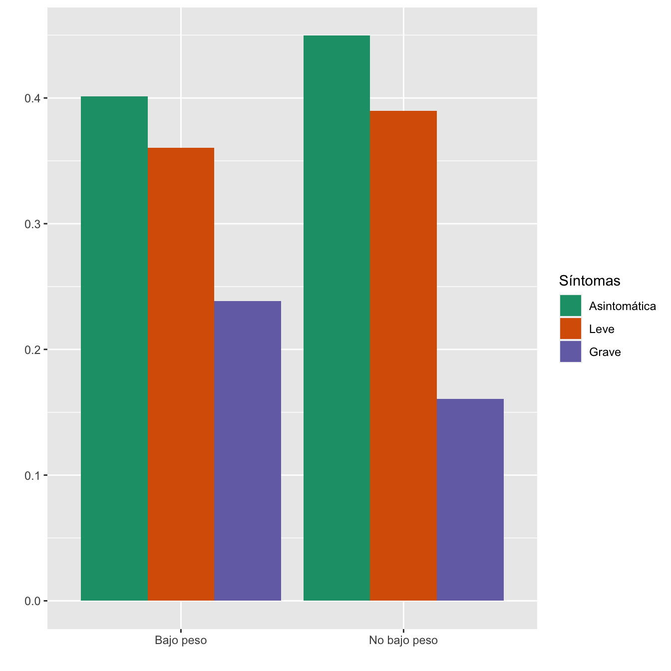
- Potencia del test: 0.634