Lección 5 Descripción global de la muestra de la segunda ola
Casos=Casos2w
Controls=Controls2w
Sint=Casos$SINTOMAS_DIAGNOSTICO
CasosGM=Casos2wGM
ControlsGM=Controls2wGM
Hay 791 infectadas y 416 no infectadas en la muestra de la segunda ola.
5.1 Antecedentes
5.1.1 Edades
data =data.frame(
  name=c(rep("Infectadas",length(I)), rep("No infectadas",length(NI))),
  Edades=c(I,NI)
  )

sample_size = data %>% group_by(name) %>% summarize(num=n())

data %>%
 left_join(sample_size) %>%
  mutate(myaxis = paste0(name, "\n", "n=", num)) %>%
  ggplot( aes(x=myaxis, y=Edades, fill=name)) +
    geom_violin(width=1) +
    geom_boxplot(width=0.1, color="black", alpha=0.2,outlier.fill="black",
               outlier.size=1) +
    theme(
      legend.position="none",
      plot.title = element_text(size=11)
    ) +
    xlab("")+
  ylab("Edades (años)")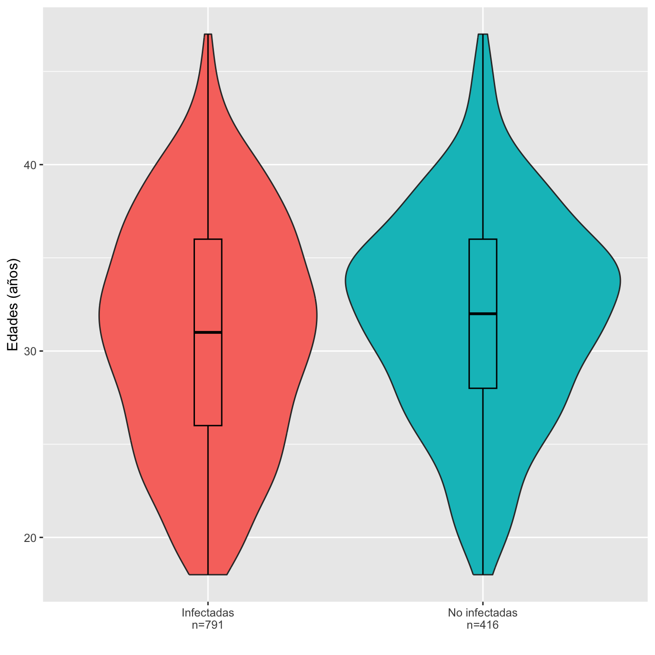
Figura 5.1:
Dades=rbind(c(min(I,na.rm=TRUE),max(I,na.rm=TRUE), round(mean(I,na.rm=TRUE),1),round(median(I,na.rm=TRUE),1),round(quantile(I,c(0.25,0.75),na.rm=TRUE),1), round(sd(I,na.rm=TRUE),1)),
            c(min(NI,na.rm=TRUE),max(NI,na.rm=TRUE), round(mean(NI,na.rm=TRUE),1),round(median(NI,na.rm=TRUE),1),round(quantile(NI,c(0.25,0.75),na.rm=TRUE),1),round(sd(NI,na.rm=TRUE),1)))

colnames(Dades)=c("Edad mínima","Edad máxima","Edad media", "Edad mediana", "1er cuartil", "3er cuartil", "Desv. típica")
rownames(Dades)=c("Infectadas", "No infectadas")

Dades %>%
  kbl() %>%
  kable_styling() %>%
scroll_box(width="100%", box_css="border: 0px;")| Edad mínima | Edad máxima | Edad media | Edad mediana | 1er cuartil | 3er cuartil | Desv. típica | |
|---|---|---|---|---|---|---|---|
| Infectadas | 18 | 47 | 30.9 | 31 | 26 | 36 | 6.2 |
| No infectadas | 18 | 47 | 31.9 | 32 | 28 | 36 | 5.6 |
Ajuste de las edades de infectadas y no infectadas a distribuciones normales: test de Shapiro-Wilks, p-valores \(10^{-6}\) y \(0.01\), respectivamente
Igualdad de edades medias: test t, p-valor 0.01, IC del 95% para la diferencia de medias [-1.66, -0.27] años
Igualdad de desviaciones típicas: test de Fligner-Killeen, p-valor \(0.00276\)
En las tablas como la que sigue:
- Los porcentajes se han calculado en la muestra sin pérdidas
- OR: la odds ratio univariante estimada de infectarse relativa a la franja de edad
- IC: el intervalo de confianza del 95% para la OR
- p-valor ajustado: p-valores de tests de Fisher bilaterales ajustados por Bonferroni calculados para la muestra sin pérdidas
I.cut=cut(I,breaks=c(0,30,40,100),labels=c("18-30","31-40",">40"))
NI.cut=cut(NI,breaks=c(0,30,40,100),labels=c("18-30","31-40",">40"))
Tabla.DMGm(I.cut,NI.cut,c("18-30","31-40",">40"))| Infectadas (N) | Infectadas (%) | No infectadas (N) | No infectadas (%) | OR | Extr. Inf. IC | Extr. Sup. IC | p-valor ajustado | |
|---|---|---|---|---|---|---|---|---|
| 18-30 | 361 | 45.7 | 151 | 37.2 | 1.42 | 1.10 | 1.83 | 0.0177 |
| 31-40 | 385 | 48.7 | 236 | 58.1 | 0.68 | 0.53 | 0.88 | 0.0076 |
| >40 | 44 | 5.6 | 19 | 4.7 | 1.20 | 0.68 | 2.21 | 1.0000 |
| Datos perdidos | 1 | 10 |
df =data.frame(
  Factor=c(rep("Infectadas",length(I)), rep("No infectadas",length(NI))),
  Edades=c( I.cut,NI.cut )
)

base=ordered(rep(c("18-30","31-40",">40"), each=2),levels=c("18-30", "31-40",   ">40"))
Grupo=rep(c("Infectada","No infectada") , length(levels(I.cut)))
valor=as.vector(prop.table(table(df), margin=1))
data <- data.frame(base,Grupo,valor)


ggplot(data, aes(fill=base , y=valor, x=Grupo)) +
  geom_bar(position="dodge", stat="identity")+
  ylab("")+
  scale_fill_brewer(palette = "Accent")+
  labs(fill = "Grupo de edad")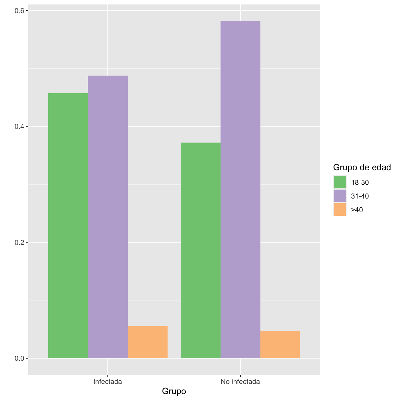
Figura 5.2:
df =data.frame(
  Factor=c(rep("Infectadas",length(I)), rep("No infectadas",length(NI))),
  Edades=c( I.cut,NI.cut )
)

base=ordered(rep(c("18-30","31-40",">40"), each=2),levels=c("18-30", "31-40",   ">40"))
Grupo=rep(c("Infectada","No infectada") , length(levels(I.cut)))
valor=as.vector(prop.table(table(df), margin=2))
data <- data.frame(base,Grupo,valor)


ggplot(data, aes(fill=Grupo, y=valor, x=base)) +
  geom_bar(position="dodge", stat="identity")+
xlab("Grupos de edad")+
  ylab("")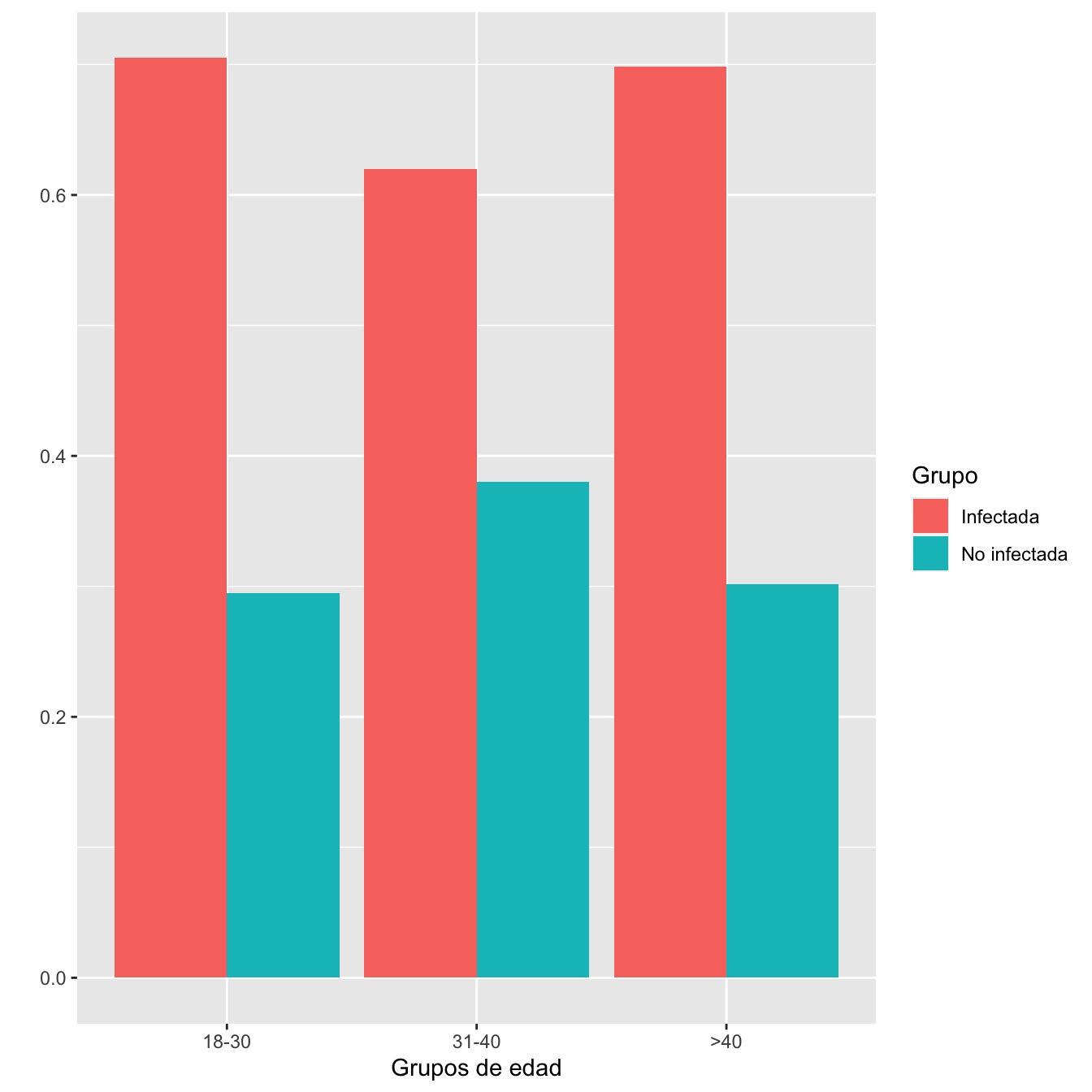
Figura 5.3:
- Igualdad de composiciones por edades de los grupos de casos y de controles: test \(\chi^2\), p-valor 0.0087.
5.1.2 Etnias
I=Casos$Etnia
I[I=="Asia"]="Asiática"
I=factor(I)
NI=factor(Controls$Etnia)
Tabla.DMGm(I,NI,c("Árabe", "Asiática", "Blanca", "Latinoamericana","Negra"),r=6)| Infectadas (N) | Infectadas (%) | No infectadas (N) | No infectadas (%) | OR | Extr. Inf. IC | Extr. Sup. IC | p-valor ajustado | |
|---|---|---|---|---|---|---|---|---|
| Árabe | 87 | 11.0 | 31 | 7.5 | 1.52 | 0.98 | 2.42 | 0.333490 |
| Asiática | 25 | 3.2 | 14 | 3.4 | 0.93 | 0.46 | 1.96 | 1.000000 |
| Blanca | 387 | 49.0 | 321 | 77.9 | 0.27 | 0.21 | 0.36 | 0.000000 |
| Latinoamericana | 265 | 33.6 | 41 | 10.0 | 4.57 | 3.18 | 6.69 | 0.000000 |
| Negra | 25 | 3.2 | 5 | 1.2 | 2.66 | 0.99 | 8.97 | 0.310083 |
| Datos perdidos | 2 | 4 |
df =data.frame(
  Factor=c(rep("Infectadas",length(I)), rep("No infectadas",length(NI))),
  Etnias=c(I,NI)
)
base=rep(levels(I) , each=2)
Grupo=rep(c("Infectada","No infectada") , length(levels(I)))
valor=as.vector(prop.table(table(df), margin=1))
data <- data.frame(base,Grupo,valor)


ggplot(data, aes(fill=base , y=valor, x=Grupo)) +
  geom_bar(position="dodge", stat="identity")+
  ylab("")+
  scale_fill_brewer(palette = "Accent")+
  labs(fill = "Etnia")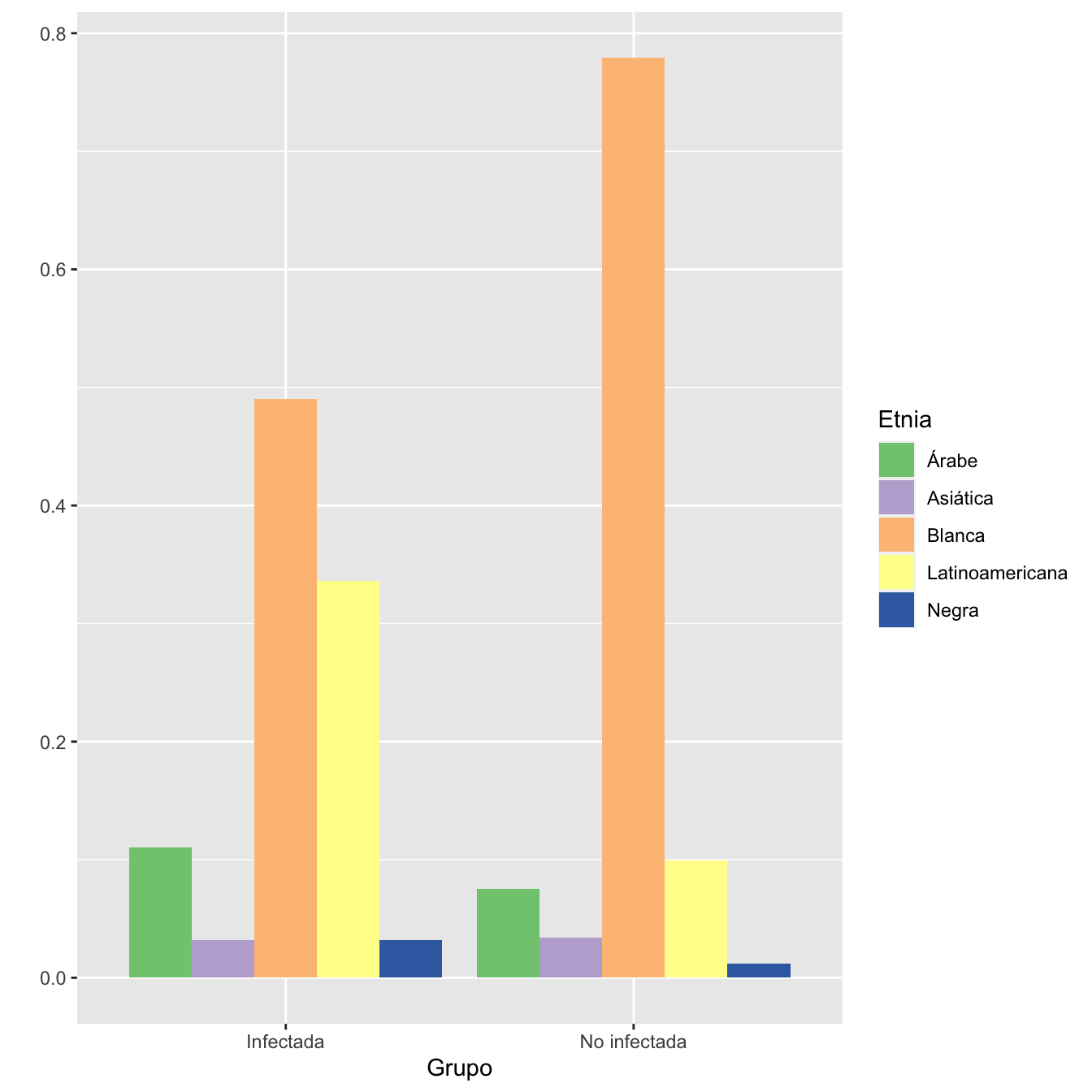
Figura 5.4:
df =data.frame(
  Factor=c(rep("Infectadas",length(I)), rep("No infectadas",length(NI))),
  Etnias=c(I,NI)
)
base=rep(levels(I) , each=2)
Grupo=rep(c("Infectada","No infectada") , length(levels(I)))
valor=as.vector(prop.table(table(df), margin=2))
data <- data.frame(base,Grupo,valor)


ggplot(data, aes(fill=Grupo, y=valor, x=base)) +
  geom_bar(position="dodge", stat="identity")+
xlab("Etnias")+
  ylab("")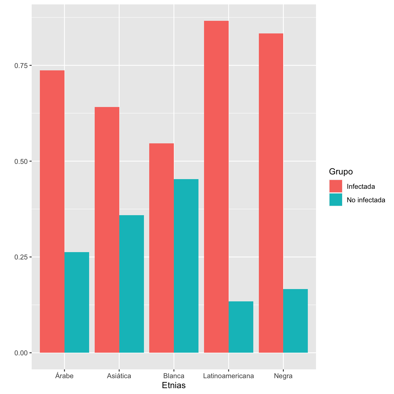
Figura 5.5:
- Composiciones por etnias de los grupos de casos y de controles: test \(\chi^2\), p-valor \(8\times 10^{-22}\)
5.1.3 Hábito tabáquico (juntando fumadoras y ex-fumadoras en una sola categoría)
En las tablas como la que sigue (para antecedentes):
- Los porcentajes se calculan para la muestra sin pérdidas
- La OR es la de infección relativa al antecedente
- El IC es el IC 95% para la OR
- El p-valor es el del test de Fisher bilateral sin tener en cuenta los datos perdidos
| Infectadas (N) | Infectadas (%) | No infectadas (N) | No infectadas (%) | OR | Extr. Inf. IC | Extr. Sup. IC | p-valor | |
|---|---|---|---|---|---|---|---|---|
| Fumadora | 57 | 7.4 | 49 | 12.7 | 0.55 | 0.36 | 0.84 | 0.0047 |
| No fumadora | 711 | 92.6 | 336 | 87.3 | ||||
| Datos perdidos | 23 | 31 |
5.1.4 Obesidad
| Infectadas (N) | Infectadas (%) | No infectadas (N) | No infectadas (%) | OR | Extr. Inf. IC | Extr. Sup. IC | p-valor | |
|---|---|---|---|---|---|---|---|---|
| Obesa | 144 | 18.2 | 51 | 13.4 | 1.44 | 1.01 | 2.08 | 0.0367 |
| No obesa | 647 | 81.8 | 331 | 86.6 | ||||
| Datos perdidos | 0 | 34 |
5.1.5 Hipertensión pregestacional
I=Casos$Hipertensión.pregestacional
NI=Controls$Hipertensión.pregestacional
Tabla.DMG(I,NI,"No HTA","HTA")| Infectadas (N) | Infectadas (%) | No infectadas (N) | No infectadas (%) | OR | Extr. Inf. IC | Extr. Sup. IC | p-valor | |
|---|---|---|---|---|---|---|---|---|
| HTA | 11 | 1.4 | 4 | 1.1 | 1.32 | 0.39 | 5.71 | 0.785 |
| No HTA | 780 | 98.6 | 374 | 98.9 | ||||
| Datos perdidos | 0 | 38 |
5.1.6 Diabetes Mellitus
| Infectadas (N) | Infectadas (%) | No infectadas (N) | No infectadas (%) | OR | Extr. Inf. IC | Extr. Sup. IC | p-valor | |
|---|---|---|---|---|---|---|---|---|
| DM | 21 | 2.7 | 11 | 2.6 | 1 | 0.46 | 2.33 | 1 |
| No DM | 770 | 97.3 | 405 | 97.4 | ||||
| Datos perdidos | 0 | 0 |
5.1.7 Enfermedades cardíacas crónicas
| Infectadas (N) | Infectadas (%) | No infectadas (N) | No infectadas (%) | OR | Extr. Inf. IC | Extr. Sup. IC | p-valor | |
|---|---|---|---|---|---|---|---|---|
| ECC | 8 | 1 | 6 | 1.6 | 0.65 | 0.2 | 2.29 | 0.4063 |
| No ECC | 783 | 99 | 381 | 98.4 | ||||
| Datos perdidos | 0 | 29 |
5.1.8 Enfermedades pulmonares crónicas (incluyendo asma)
INA=Casos$Enfermedad.pulmonar.crónica.no.asma
NINA=Controls$Enfermedad.pulmonar.crónica.no.asma
NINA[NINA==0]="No"
NINA[NINA==1]="Sí"
IA=Casos$Diagnóstico.clínico.de.Asma
NIA=Controls$Diagnóstico.clínico.de.Asma
NIA[NIA==0]="No"
NIA[NIA==1]="Sí"

I=rep(NA,n_I)
for (i in 1:n_I){I[i]=max(INA[i],IA[i],na.rm=TRUE)}
NI=rep(NA,n_NI)
for (i in 1:n_NI){NI[i]=max(NINA[i],NIA[i],na.rm=TRUE)}
NI[NI==-Inf]=NA


Tabla.DMG(I,NI,"No EPC","EPC")| Infectadas (N) | Infectadas (%) | No infectadas (N) | No infectadas (%) | OR | Extr. Inf. IC | Extr. Sup. IC | p-valor | |
|---|---|---|---|---|---|---|---|---|
| EPC | 36 | 4.6 | 12 | 3.1 | 1.49 | 0.75 | 3.19 | 0.2738 |
| No EPC | 755 | 95.4 | 376 | 96.9 | ||||
| Datos perdidos | 877 | 1219 |
5.1.9 Paridad
| Infectadas (N) | Infectadas (%) | No infectadas (N) | No infectadas (%) | OR | Extr. Inf. IC | Extr. Sup. IC | p-valor | |
|---|---|---|---|---|---|---|---|---|
| Nulípara | 287 | 36.4 | 193 | 46.7 | 0.65 | 0.51 | 0.84 | 6e-04 |
| Multípara | 502 | 63.6 | 220 | 53.3 | ||||
| Datos perdidos | 2 | 3 |
5.1.10 Gestación múltiple
I=Casos$Gestación.Múltiple
NI=Controls$Gestación.Múltiple
Tabla.DMG(I,NI,"Gestación única","Gestación múltiple")| Infectadas (N) | Infectadas (%) | No infectadas (N) | No infectadas (%) | OR | Extr. Inf. IC | Extr. Sup. IC | p-valor | |
|---|---|---|---|---|---|---|---|---|
| Gestación múltiple | 13 | 1.6 | 6 | 1.4 | 1.14 | 0.4 | 3.69 | 1 |
| Gestación única | 778 | 98.4 | 410 | 98.6 | ||||
| Datos perdidos | 0 | 0 |
5.2 Desenlaces
5.2.1 Anomalías congénitas
En las tablas como la que sigue (para desenlaces):
- Los porcentajes se calculan para la muestra sin pérdidas
- RA y RR: riesgo absoluto y relativo del desenlace relativo a la infección
- Los IC son el IC 95% para RA y RR
- El p-valor es el del test de Fisher bilateral sin tener en cuenta los datos perdidos
I=Casos$Diagnóstico.de.malformación.ecográfica._.semana.20._
NI=Controls$Diagnóstico.de.malformación.ecográfica._.semana.20._
Tabla.DMGC(I,NI,"No anomalía congénita","Anomalía congénita")| Infectadas (N) | Infectadas (%) | No infectadas (N) | No infectadas (%) | RA | Extr. Inf. IC RA | Extr. Sup. IC RA | RR | Extr. Inf. IC RA | Extr. Sup. IC RR | p-valor | |
|---|---|---|---|---|---|---|---|---|---|---|---|
| Anomalía congénita | 14 | 1.8 | 4 | 1 | 0.0085 | -0.0069 | 0.0239 | 1.86 | 0.65 | 5.37 | 0.3248 |
| No anomalía congénita | 750 | 98.2 | 403 | 99 | |||||||
| Datos perdidos | 27 | 9 |
5.2.2 Retraso del crecimiento intrauterino
I=Casos$Defecto.del.crecimiento.fetal..en.tercer.trimestre._.CIR._.
NI=Controls$Defecto.del.crecimiento.fetal..en.tercer.trimestre._.CIR._.
Tabla.DMGC(I,NI,"No RCIU","RCIU")| Infectadas (N) | Infectadas (%) | No infectadas (N) | No infectadas (%) | RA | Extr. Inf. IC RA | Extr. Sup. IC RA | RR | Extr. Inf. IC RA | Extr. Sup. IC RR | p-valor | |
|---|---|---|---|---|---|---|---|---|---|---|---|
| RCIU | 27 | 3.4 | 11 | 2.7 | 0.0073 | -0.0147 | 0.0293 | 1.27 | 0.65 | 2.51 | 0.6029 |
| No RCIU | 764 | 96.6 | 399 | 97.3 | |||||||
| Datos perdidos | 0 | 6 |
5.2.3 Diabetes gestacional
| Infectadas (N) | Infectadas (%) | No infectadas (N) | No infectadas (%) | RA | Extr. Inf. IC RA | Extr. Sup. IC RA | RR | Extr. Inf. IC RA | Extr. Sup. IC RR | p-valor | |
|---|---|---|---|---|---|---|---|---|---|---|---|
| DG | 59 | 7.5 | 41 | 10 | -0.0254 | -0.0616 | 0.0108 | 0.75 | 0.51 | 1.09 | 0.1518 |
| No DG | 732 | 92.5 | 369 | 90 | |||||||
| Datos perdidos | 0 | 6 |
5.2.4 Hipertensión gestacional
| Infectadas (N) | Infectadas (%) | No infectadas (N) | No infectadas (%) | RA | Extr. Inf. IC RA | Extr. Sup. IC RA | RR | Extr. Inf. IC RA | Extr. Sup. IC RR | p-valor | |
|---|---|---|---|---|---|---|---|---|---|---|---|
| HG | 22 | 2.8 | 7 | 1.7 | 0.0107 | -0.0081 | 0.0296 | 1.63 | 0.72 | 3.7 | 0.3226 |
| No HG | 769 | 97.2 | 403 | 98.3 | |||||||
| Datos perdidos | 0 | 6 |
5.2.5 Preeclampsia
| Infectadas (N) | Infectadas (%) | No infectadas (N) | No infectadas (%) | RA | Extr. Inf. IC RA | Extr. Sup. IC RA | RR | Extr. Inf. IC RA | Extr. Sup. IC RR | p-valor | |
|---|---|---|---|---|---|---|---|---|---|---|---|
| PE | 40 | 5.1 | 8 | 1.9 | 0.0313 | 0.0093 | 0.0534 | 2.63 | 1.27 | 5.49 | 0.0079 |
| No PE | 751 | 94.9 | 408 | 98.1 | |||||||
| Datos perdidos | 0 | 0 |
5.2.6 Preeclampsia con criterios de gravedad
n_PI=sum(Casos$PREECLAMPSIA_ECLAMPSIA_TOTAL)
n_PNI=sum(Controls$PREECLAMPSIA)
I=Casos[Casos$PREECLAMPSIA_ECLAMPSIA_TOTAL==1,]$Preeclampsia.grave_HELLP_ECLAMPSIA

NI1=Controls[Controls$PREECLAMPSIA==1,]$preeclampsia_severa
NI2=Controls[Controls$PREECLAMPSIA==1,]$Preeclampsia.grave.No.HELLP
NI=rep(NA,n_PNI)
for (i in 1:n_PNI){NI[i]=max(NI1[i],NI2[i],na.rm=TRUE)}

Tabla.DMGCr(I,NI,"PE sin CG","PE con CG",n_PI,n_PNI)| Infectadas (N) | Infectadas (%) | No infectadas (N) | No infectadas (%) | RA | Extr. Inf. IC RA | Extr. Sup. IC RA | RR | Extr. Inf. IC RA | Extr. Sup. IC RR | p-valor | |
|---|---|---|---|---|---|---|---|---|---|---|---|
| PE con CG | 11 | 27.5 | 3 | 37.5 | -0.1 | -0.5379 | 0.3379 | 0.73 | 0.31 | 2.2 | 0.6757 |
| PE sin CG | 29 | 72.5 | 5 | 62.5 | |||||||
| Datos perdidos | 0 | 0 |
5.2.7 Rotura prematura de membranas
| Infectadas (N) | Infectadas (%) | No infectadas (N) | No infectadas (%) | RA | Extr. Inf. IC RA | Extr. Sup. IC RA | RR | Extr. Inf. IC RA | Extr. Sup. IC RR | p-valor | |
|---|---|---|---|---|---|---|---|---|---|---|---|
| RPM | 111 | 14 | 49 | 11.8 | 0.0225 | -0.0186 | 0.0637 | 1.19 | 0.87 | 1.63 | 0.2852 |
| No RPM | 680 | 86 | 367 | 88.2 | |||||||
| Datos perdidos | 0 | 0 |
5.2.8 Edad gestacional en el momento del parto
Dades=round(rbind(c(min(I,na.rm=TRUE),max(I,na.rm=TRUE), round(mean(I,na.rm=TRUE),1),round(median(I,na.rm=TRUE),1),round(quantile(I,c(0.25,0.75),na.rm=TRUE),1), round(sd(I,na.rm=TRUE),1)),
            c(min(NI,na.rm=TRUE),max(NI,na.rm=TRUE), round(mean(NI,na.rm=TRUE),1),round(median(NI,na.rm=TRUE),1),round(quantile(NI,c(0.25,0.75),na.rm=TRUE),1),round(sd(NI,na.rm=TRUE),1))),1)

colnames(Dades)=c("Edad gest. mínima","Edad gest. máxima","Edad gest. media", "Edad gest. mediana", "1er cuartil", "3er cuartil", "Desv. típica")
rownames(Dades)=c("Infectadas", "No infectadas")

Dades %>%
  kbl() %>%
  kable_styling() %>%
scroll_box(width="100%", box_css="border: 0px;")| Edad gest. mínima | Edad gest. máxima | Edad gest. media | Edad gest. mediana | 1er cuartil | 3er cuartil | Desv. típica | |
|---|---|---|---|---|---|---|---|
| Infectadas | 18 | 42.1 | 39.1 | 39.4 | 38.4 | 40.4 | 2.2 |
| No infectadas | 23 | 42.0 | 39.4 | 39.6 | 38.9 | 40.4 | 1.7 |
data =data.frame(
  name=c( rep("Infectadas",length(I)), rep("No infectadas",length(NI))),
  Edades=c( I,NI )
)

data %>%
  ggplot( aes(x=name, y=Edades, fill=name)) +
    geom_violin(width=1) +
    geom_boxplot(width=0.1, color="black", alpha=0.2,outlier.fill="black",
               outlier.size=1) +
    theme(
      legend.position="none",
      plot.title = element_text(size=11)
    ) +
    xlab("")+
  ylab("Edades gestacionales (semanas)")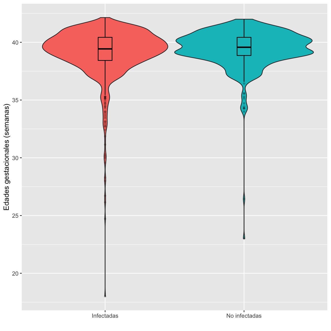
Figura 5.6:
Ajuste de las edades gestacionales de infectadas y no infectadas a distribuciones normales: test de Shapiro-Wilks, p-valores \(4\times 10^{-32}\) y \(2\times 10^{-23}\), respectivamente
Edades gestacionales medias: test t, p-valor \(0.008\), IC del 95% para la diferencia de medias [-0.53, -0.08]
Desviaciones típicas: test de Fligner-Killeen, p-valor \(0.02\)
Nota: Como vemos en los boxplot, hay dos casos de infectadas con edades gestacionales incompatibles con la definición de “parto” (y que además luego tienen información incompatible con esto). Son 00133-00046 y 00268-00008. Si las quitamos, las conclusiones son las mismas:
Ajuste de las edades gestacionales de infectadas y no infectadas a distribuciones normales: test de Shapiro-Wilks, p-valores \(10^{-29}\) y \(2\times 10^{-23}\), respectivamente
Edades medias: test t, p-valor \(0.01\), IC del 95% para la diferencia de medias [-0.5, -0.06]
Desviaciones típicas: test de Fligner-Killeen, p-valor \(0.02\)
5.2.9 Prematuridad
| Infectadas (N) | Infectadas (%) | No infectadas (N) | No infectadas (%) | RA | Extr. Inf. IC RA | Extr. Sup. IC RA | RR | Extr. Inf. IC RA | Extr. Sup. IC RR | p-valor | |
|---|---|---|---|---|---|---|---|---|---|---|---|
| Prematuro | 65 | 8.2 | 19 | 4.6 | 0.0365 | 0.0069 | 0.0661 | 1.8 | 1.1 | 2.95 | 0.0173501 |
| No prematuro | 726 | 91.8 | 397 | 95.4 | |||||||
| Datos perdidos | 0 | 0 |
5.2.10 Eventos trombóticos
I=Casos$EVENTOS_TROMBO_TOTALES
NI1=Controls$DVT
NI2=Controls$PE
NI=rep(NA,n_NI)
for (i in 1:n_NI){NI[i]=max(NI1[i],NI2[i],na.rm=TRUE)}
NI=factor(NI,levels=0:1)

Tabla.DMGC(I,NI,"No eventos trombóticos","Eventos trombóticos")| Infectadas (N) | Infectadas (%) | No infectadas (N) | No infectadas (%) | RA | Extr. Inf. IC RA | Extr. Sup. IC RA | RR | Extr. Inf. IC RA | Extr. Sup. IC RR | p-valor | |
|---|---|---|---|---|---|---|---|---|---|---|---|
| Eventos trombóticos | 5 | 0.6 | 2 | 0.5 | 0.0015 | -0.0086 | 0.0117 | 1.31 | 0.3 | 5.86 | 1 |
| No eventos trombóticos | 786 | 99.4 | 414 | 99.5 | |||||||
| Datos perdidos | 0 | 1191 |
5.2.11 Eventos hemorrágicos
I=Casos$EVENTOS_HEMORRAGICOS_TOTAL
NI=Controls$eventos_hemorragicos
Tabla.DMGC(I,NI,"No eventos heomorrágicos","Eventos hemorrágicos")| Infectadas (N) | Infectadas (%) | No infectadas (N) | No infectadas (%) | RA | Extr. Inf. IC RA | Extr. Sup. IC RA | RR | Extr. Inf. IC RA | Extr. Sup. IC RR | p-valor | |
|---|---|---|---|---|---|---|---|---|---|---|---|
| Eventos hemorrágicos | 40 | 5.1 | 25 | 6 | -0.0095 | -0.0388 | 0.0198 | 0.84 | 0.52 | 1.36 | 0.5037 |
| No eventos heomorrágicos | 751 | 94.9 | 391 | 94 | |||||||
| Datos perdidos | 0 | 0 |
5.2.12 Ingreso materno en UCI
| Infectadas (N) | Infectadas (%) | No infectadas (N) | No infectadas (%) | RA | Extr. Inf. IC RA | Extr. Sup. IC RA | RR | Extr. Inf. IC RA | Extr. Sup. IC RR | p-valor | |
|---|---|---|---|---|---|---|---|---|---|---|---|
| UCI | 13 | 1.6 | 0 | 0 | 0.0164 | 0.0057 | 0.0271 | Inf | 1.79 | Inf | 0.0060658 |
| No UCI | 778 | 98.4 | 416 | 100 | |||||||
| Datos perdidos | 0 | 0 |
5.2.13 Ingreso materno en UCI según el momento del parto o cesárea
UCI.I=sum(Casos$UCI,na.rm=TRUE)
UCI.NI=sum(Controls$UCI...9,na.rm=TRUE)
I=Casos$UCI_ANTES.DESPUES.DEL.PARTO
NI=Controls$UCI.ANTES.DEL.PARTO  #Vacía
NA_I=length(I[is.na(I)])
NA_NI=length(NI[is.na(NI)])

EE=rbind(as.vector(table(I)),
         c(0,UCI.NI))
EEExt=rbind(c(as.vector(table(I)),0),
            round(100*c(as.vector(table(I)),0)/UCI.I,1),
            c(0,UCI.NI,0),
            c(0,100,0))
rownames(EEExt)=Columnes

colnames(EEExt)=c("UCI antes del parto", " UCI después del parto","Pérdidas")


t(EEExt) %>%
  kbl() %>%
kable_styling()| Infectadas (N) | Infectadas (%) | No infectadas (N) | No infectadas (%) | |
|---|---|---|---|---|
| UCI antes del parto | 6 | 46.2 | 0 | 0 |
| UCI después del parto | 7 | 53.8 | 0 | 100 |
| Pérdidas | 0 | 0.0 | 0 | 0 |
Al no haber ingresos en UCI en no infectadas, no tiene sentido comparar proprociones
5.2.14 Embarazos con algún feto muerto anteparto
I=Casos$Feto.muerto.intraútero
I[I=="Sí"]=1
I[I=="No"]=0
NI1=Controls$Feto.vivo...194
NI1[NI1=="Sí"]=0
NI1[NI1=="No"]=1
NI2=Controls$Feto.vivo...245
NI2[NI2=="Sí"]=0
NI2[NI2=="No"]=1
NI=NI1
for (i in 1:length(NI1)){NI[i]=max(NI1[i],NI2[i],na.rm=TRUE)}
NI=factor(NI,levels=c(0,1))

Tabla.DMGC(I,NI,"Ningún feto muerto anteparto","Algún feto muerto anteparto")| Infectadas (N) | Infectadas (%) | No infectadas (N) | No infectadas (%) | RA | Extr. Inf. IC RA | Extr. Sup. IC RA | RR | Extr. Inf. IC RA | Extr. Sup. IC RR | p-valor | |
|---|---|---|---|---|---|---|---|---|---|---|---|
| Algún feto muerto anteparto | 10 | 1.3 | 0 | 0 | 0.0126 | 0.003 | 0.0223 | Inf | 1.38 | Inf | 0.0185 |
| Ningún feto muerto anteparto | 781 | 98.7 | 416 | 100 | |||||||
| Datos perdidos | 0 | 0 |
5.2.15 Inicio del parto
I=Casos$Inicio.de.parto
I=factor(Casos$Inicio.de.parto,levels=c("Espontáneo", "Inducido", "Cesárea"),ordered=TRUE)
NI=Controls$Inicio.de.parto
NI[NI=="Cesárea programada"]="Cesárea"
NI=factor(NI,levels=c("Espontáneo", "Inducido", "Cesárea"),ordered=TRUE)

Tabla.DMGCm(I,NI,c("Espontáneo", "Inducido", "Cesárea"),r=9)| Infectadas (N) | Infectadas (%) | No infectadas (N) | No infectadas (%) | RA | Extr. Inf. IC RA | Extr. Sup. IC RA | RR | Extr. Inf. IC RA | Extr. Sup. IC RR | p-valor | |
|---|---|---|---|---|---|---|---|---|---|---|---|
| Espontáneo | 429 | 54.2 | 266 | 63.9 | -0.0971 | -0.1567 | -0.0375 | 0.848 | 0.770 | 0.934 | 0.0035207 |
| Inducido | 303 | 38.3 | 129 | 31.0 | 0.0730 | 0.0152 | 0.1307 | 1.235 | 1.044 | 1.461 | 0.0410927 |
| Cesárea | 59 | 7.5 | 21 | 5.0 | 0.0241 | -0.0056 | 0.0538 | 1.478 | 0.915 | 2.385 | 0.3451086 |
| Datos perdidos | 0 | 0 |
df =data.frame(
  Factor=c( rep("Infectadas",length(I)), rep("No infectadas",length(NI))),
  Inicios=ordered(c( I,NI ),levels=c("Espontáneo","Inducido","Cesárea"))
)

base=ordered(rep(c("Espontáneo","Inducido","Cesárea"), each=2),levels=c("Espontáneo","Inducido","Cesárea"))
Grupo=rep(c("Infectada","No infectada") , 3)
valor=c(as.vector(prop.table(table(df),margin=1))                 )
data <- data.frame(base,Grupo,valor)


ggplot(data, aes(fill=base, y=valor, x=Grupo)) +
  geom_bar(position="dodge", stat="identity")+
  ylab("")+
  scale_fill_brewer(palette = "Set3")+
  labs(fill = "Inicio de parto")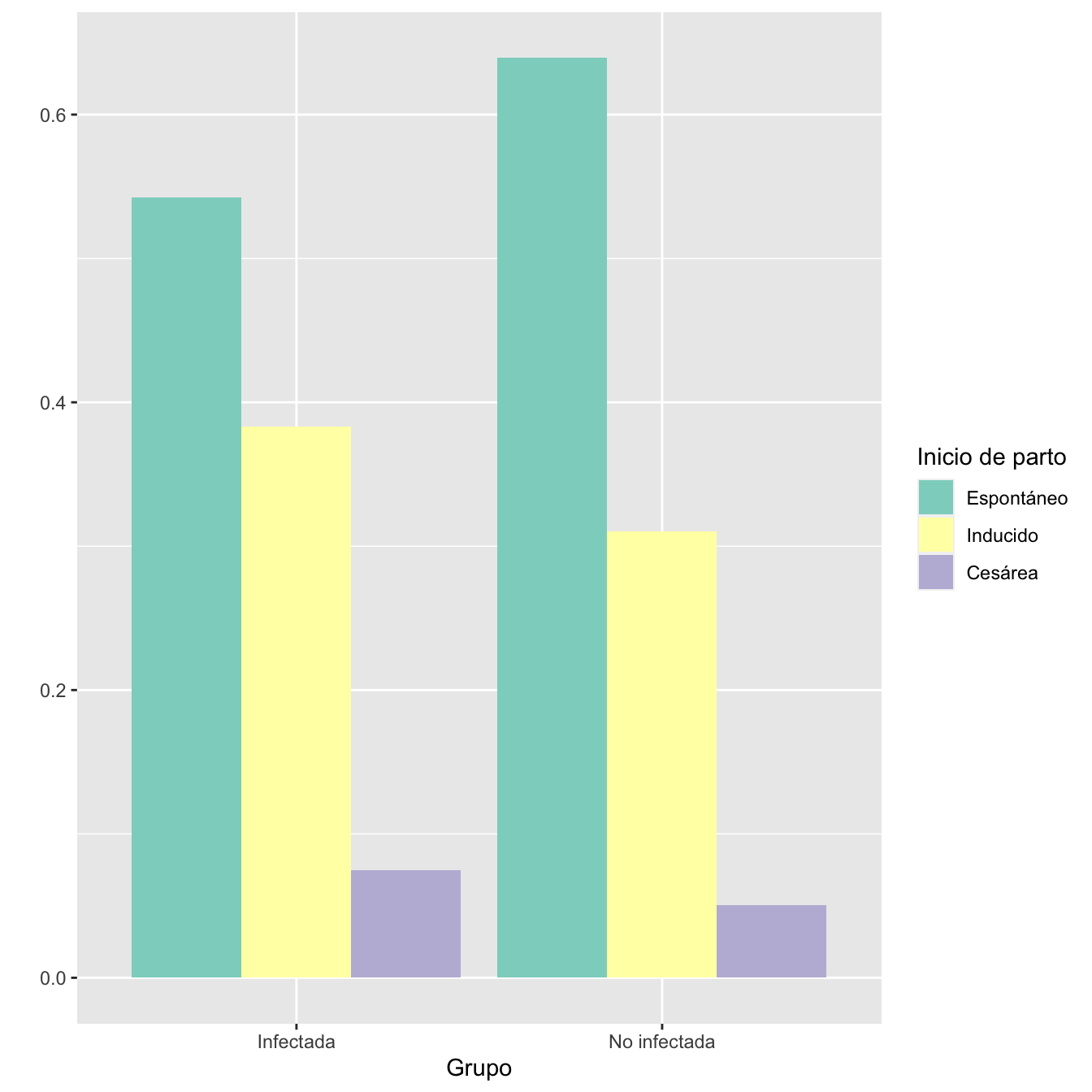
Figura 5.7:
df =data.frame(
  Factor=c( rep("Infectadas",length(I)), rep("No infectadas",length(NI))),
  Inicios=ordered(c( I,NI ),levels=c("Espontáneo","Inducido","Cesárea"))
)

base=ordered(rep(c("Espontáneo","Inducido","Cesárea"), each=2),levels=c("Espontáneo","Inducido","Cesárea"))
Grupo=rep(c("Infectada","No infectada") , 3)
valor=c(as.vector(prop.table(table(df),margin=2))                 )
data <- data.frame(base,Grupo,valor)


ggplot(data, aes(fill=Grupo, y=valor, x=base)) +
  geom_bar(position="dodge", stat="identity")+
  xlab("Inicios de parto")+
  ylab("")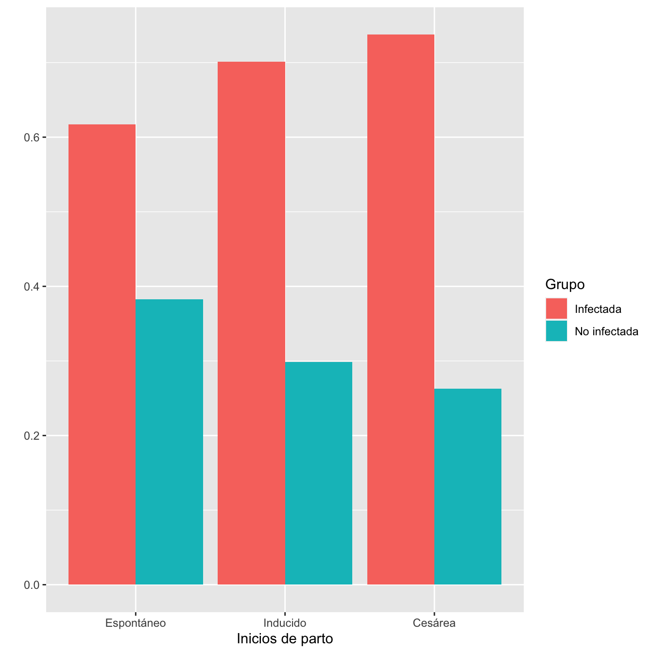
Figura 5.8:
- Distribuciones de los inicios de parto en los grupos de infectadas y no infectadas: test \(\chi^2\), p-valor \(0.004\)
5.2.16 Tipo de parto
I.In=Casos$Inicio.de.parto
I.In[I.In=="Cesárea"]="Cesárea programada"
I=Casos$Tipo.de.parto
I[I.In=="Cesárea programada"]="Cesárea programada"
I[I=="Cesárea"]="Cesárea urgente"
I[I=="Eutocico"]="Eutócico"
I=factor(I,levels=c("Eutócico", "Instrumental", "Cesárea programada", "Cesárea urgente"),ordered=TRUE)

NI.In=Controls$Inicio.de.parto
NI=Controls$Tipo.de.parto
NI[NI.In=="Cesárea programada"]="Cesárea programada"
NI[NI=="Cesárea"]="Cesárea urgente"
NI[NI=="Eutocico"]="Eutócico"
NI=factor(NI,levels=c("Eutócico", "Instrumental", "Cesárea programada", "Cesárea urgente"),ordered=TRUE)

Tabla.DMGCm(I,NI,c("Eutócico", "Instrumental", "Cesárea programada", "Cesárea urgente"),r=6)| Infectadas (N) | Infectadas (%) | No infectadas (N) | No infectadas (%) | RA | Extr. Inf. IC RA | Extr. Sup. IC RA | RR | Extr. Inf. IC RA | Extr. Sup. IC RR | p-valor | |
|---|---|---|---|---|---|---|---|---|---|---|---|
| Eutócico | 527 | 66.6 | 277 | 66.6 | 0.0004 | -0.0560 | 0.0567 | 1.001 | 0.920 | 1.088 | 1.000000 |
| Instrumental | 77 | 9.7 | 58 | 13.9 | -0.0421 | -0.0831 | -0.0011 | 0.698 | 0.508 | 0.960 | 0.136716 |
| Cesárea programada | 59 | 7.5 | 21 | 5.0 | 0.0241 | -0.0056 | 0.0538 | 1.478 | 0.915 | 2.385 | 0.460145 |
| Cesárea urgente | 128 | 16.2 | 60 | 14.4 | 0.0176 | -0.0267 | 0.0618 | 1.122 | 0.847 | 1.487 | 1.000000 |
| Datos perdidos | 0 | 0 |
df =data.frame(
  Factor=c( rep("Infectadas",length(I)), rep("No infectadas",length(NI))),
  Inicios=ordered(c( I,NI ),levels=c("Eutócico", "Instrumental", "Cesárea programada", "Cesárea urgente"))
)

base=ordered(rep(c("Eutócico", "Instrumental", "Cesárea prog.", "Cesárea urg."), each=2),levels=c("Eutócico", "Instrumental", "Cesárea prog.", "Cesárea urg."))
Grupo=rep(c("Infectada","No infectada") , 4)
valor=c(as.vector(prop.table(table(df),margin=1))                 )
data <- data.frame(base,Grupo,valor)


ggplot(data, aes(fill=base, y=valor, x=Grupo)) +
  geom_bar(position="dodge", stat="identity")+
  ylab("")+
  scale_fill_brewer(palette = "Set3")+
  labs(fill = "Tipo de parto")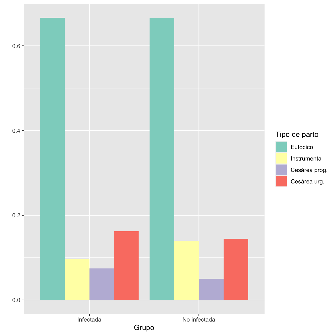
Figura 5.9:
df =data.frame(
  Factor=c( rep("Infectadas",length(I)), rep("No infectadas",length(NI))),
  Inicios=ordered(c( I,NI ),levels=c("Eutócico", "Instrumental", "Cesárea programada", "Cesárea urgente"))
)

base=ordered(rep(c("Eutócico", "Instrumental", "Cesárea prog.", "Cesárea urg."), each=2),levels=c("Eutócico", "Instrumental", "Cesárea prog.", "Cesárea urg."))
Grupo=rep(c("Infectada","No infectada") , 4)
valor=as.vector(prop.table(table(df), margin=2))
data <- data.frame(base,Grupo,valor)


ggplot(data, aes(fill=Grupo, y=valor, x=base)) +
  geom_bar(position="dodge", stat="identity")+
  xlab("Tipos de parto")+
  ylab("")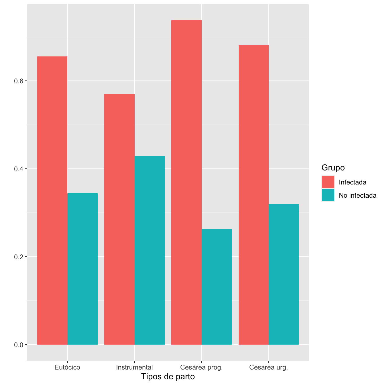
Figura 5.10:
- Distribuciones de los tipos de parto en los grupos de infectadas y no infectadas: test \(\chi^2\), p-valor \(0.06\)
5.2.17 Hemorragias postparto
I=Casos$Hemorragia.postparto
I.sino=I
I.sino[!is.na(I.sino)& I.sino!="No"]="Sí"


NI=Controls$Hemorragia.postparto
NI.sino=NI
NI.sino[!is.na(NI.sino)& NI.sino!="No"]="Sí"

Tabla.DMGC(I.sino,NI.sino,"No HPP","HPP")| Infectadas (N) | Infectadas (%) | No infectadas (N) | No infectadas (%) | RA | Extr. Inf. IC RA | Extr. Sup. IC RA | RR | Extr. Inf. IC RA | Extr. Sup. IC RR | p-valor | |
|---|---|---|---|---|---|---|---|---|---|---|---|
| HPP | 32 | 4.1 | 20 | 4.9 | -0.0075 | -0.0343 | 0.0194 | 0.85 | 0.49 | 1.45 | 0.5535 |
| No HPP | 747 | 95.9 | 392 | 95.1 | |||||||
| Datos perdidos | 12 | 4 |
| Infectadas (N) | Infectadas (%) | No infectadas (N) | No infectadas (%) | RA | Extr. Inf. IC RA | Extr. Sup. IC RA | RR | Extr. Inf. IC RA | Extr. Sup. IC RR | p-valor | |
|---|---|---|---|---|---|---|---|---|---|---|---|
| HPP tratamiento médico | 27 | 3.5 | 17 | 4.1 | -0.0066 | -0.0316 | 0.0184 | 0.840 | 0.467 | 1.511 | 1 |
| HPP tratamiento quirúrgico conservador | 5 | 0.6 | 3 | 0.7 | -0.0009 | -0.0117 | 0.0099 | 0.881 | 0.232 | 3.349 | 1 |
| No | 747 | 95.9 | 392 | 95.1 | 0.0075 | -0.0194 | 0.0343 | 1.008 | 0.982 | 1.034 | 1 |
| Datos perdidos | 12 | 4 |
df =data.frame(
  Factor=c( rep("Infectadas",length(I[I!="No"])), rep("No infectadas",length(NI[NI!="No"]))),
  Hemos=ordered(c( I[I!="No"],NI[NI!="No"] ),levels=names(table(I))[-4])
)

base=ordered(rep(c("Tto. médico", "Tto. Qx conservador"), each=2),levels=c("Tto. médico", "Tto. Qx conservador"))
Grupo=rep(c("Infectada","No infectada") , 2)
valor=as.vector(prop.table(table(df)[,1:2], margin=1))
data <- data.frame(base,Grupo,valor)


ggplot(data, aes(fill=Grupo, y=valor, x=base)) +
  geom_bar(position="dodge", stat="identity")+
  xlab("Tratamientos de hemorragia postparto")+
  ylab("")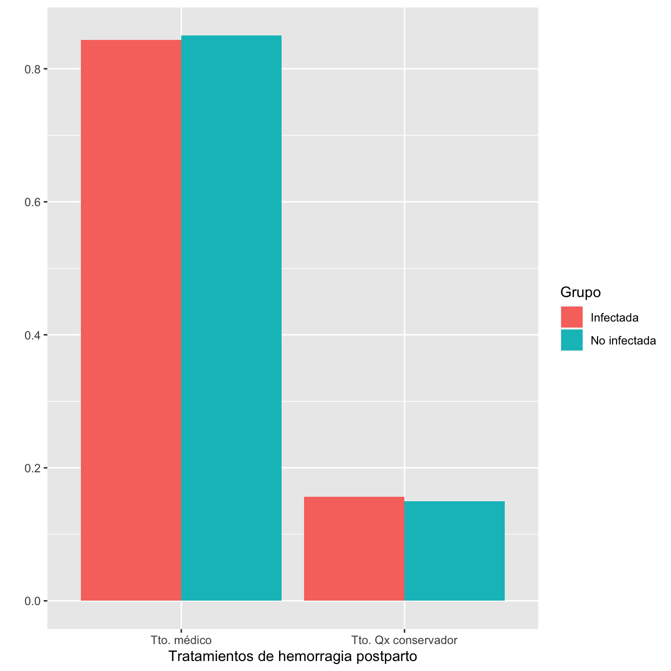
Figura 5.11:
Distribuciones de los tipos de hemorragia postparto (incluyendo Noes) en los grupos de infectadas y no infectadas: test \(\chi^2\) de Montercarlo, p-valor 0.86
Distribuciones de los tipos de hemorragia postparto en los grupos de infectadas y no infectadas que tuvieron hemorragia postparto: test \(\chi^2\) de Montercarlo, p-valor NaN
5.2.18 Fetos muertos anteparto
I1=Casos$Feto.muerto.intraútero
I1[I1=="Sí"]="Muerto"
I1[I1=="No"]="Vivo"
I2=CasosGM$Feto.vivo
I2[I2=="Sí"]="Vivo"
I2[I2=="No"]="Muerto"
I=c(I1,I2)
I=ordered(I,levels=c("Vivo","Muerto"))


n_IFT=length(I)
n_VI=as.vector(table(I))[1]NI1=Controls$Feto.vivo...194
NI2=ControlsGM$Feto.vivo...245
NI=c(NI1,NI2)
NI[NI=="Sí"]="Vivo"
NI[NI=="No"]="Muerto"
NI=ordered(NI,levels=c("Vivo","Muerto"))
n_NIFT=length(NI)
n_VNI=as.vector(table(NI))[1]
Tabla.DMGC(I,NI,"Feto vivo","Feto muerto anteparto")| Infectadas (N) | Infectadas (%) | No infectadas (N) | No infectadas (%) | RA | Extr. Inf. IC RA | Extr. Sup. IC RA | RR | Extr. Inf. IC RA | Extr. Sup. IC RR | p-valor | |
|---|---|---|---|---|---|---|---|---|---|---|---|
| Feto muerto anteparto | 10 | 1.2 | 0 | 0 | 0.0124 | 0.003 | 0.0219 | Inf | 1.38 | Inf | 0.0186 |
| Feto vivo | 794 | 98.8 | 422 | 100 | |||||||
| Datos perdidos | 0 | 0 |
5.2.19 Peso de neonatos al nacimiento
I=c(Casos[Casos$Feto.muerto.intraútero=="No",]$Peso._gramos_...125,CasosGM[CasosGM$Feto.vivo=="Sí",]$Peso._gramos_...148)
NI=c(Controls[Controls$Feto.vivo...194=="Sí",]$Peso._gramos_...198,ControlsGM[ControlsGM$Feto.vivo...245=="Sí",]$Peso._gramos_...247)
data =data.frame(
name=c(rep("Hijos de infectadas",length(I)), rep("Hijos de no infectadas",length(NI))),
Pesos=c(I,NI)
)
sample_size = data %>% group_by(name) %>% summarize(num=n())
data %>%
left_join(sample_size) %>%
mutate(myaxis = paste0(name, "\n", "n=", num)) %>%
ggplot( aes(x=myaxis, y=Pesos, fill=name)) +
geom_violin(width=0.9) +
geom_boxplot(width=0.1, color="black", alpha=0.2,outlier.fill="black",
outlier.size=1) +
theme(
legend.position="none",
plot.title = element_text(size=11)
) +
xlab("")+
ylab("Pesos (gramos)")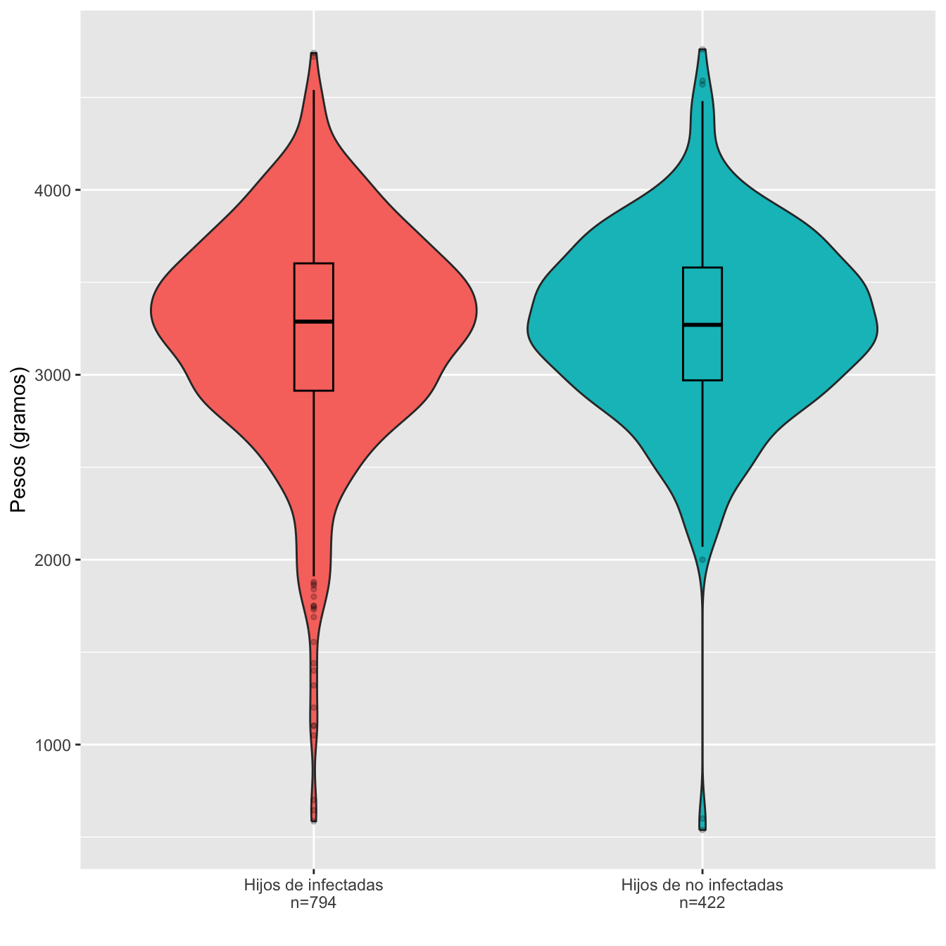
Figura 5.12:
Dades=rbind(c(min(I,na.rm=TRUE),max(I,na.rm=TRUE), round(mean(I,na.rm=TRUE),1),round(median(I,na.rm=TRUE),1),round(quantile(I,c(0.25,0.75),na.rm=TRUE),1), round(sd(I,na.rm=TRUE),1)),
            c(min(NI,na.rm=TRUE),max(NI,na.rm=TRUE), round(mean(NI,na.rm=TRUE),1),round(median(NI,na.rm=TRUE),1),round(quantile(NI,c(0.25,0.75),na.rm=TRUE),1),round(sd(NI,na.rm=TRUE),1)))

colnames(Dades)=c("Peso mínimo","Peso máximo","Peso medio", "Peso mediano", "1er cuartil", "3er cuartil", "Desv. típica")
rownames(Dades)=c("Infectadas", "No infectadas")

Dades %>%
  kbl() %>%
  kable_styling() %>%
scroll_box(width="100%", box_css="border: 0px;")| Peso mínimo | Peso máximo | Peso medio | Peso mediano | 1er cuartil | 3er cuartil | Desv. típica | |
|---|---|---|---|---|---|---|---|
| Infectadas | 585 | 4740 | 3229.0 | 3287.5 | 2913.8 | 3602.5 | 587.1 |
| No infectadas | 538 | 4760 | 3265.7 | 3270.0 | 2970.0 | 3580.0 | 503.6 |
Ajuste de los pesos de hijos de infectadas y no infectadas a distribuciones normales: test de Shapiro-Wilks, p-valores \(7\times 10^{-13}\) y \(3\times 10^{-8}\), respectivamente
Pesos medios: test t, p-valor 0.2597, IC del 95% para la diferencia de medias [-100.5, 27.15]
Desviaciones típicas: test de Fligner-Killeen, p-valor 0.0129
Definimos bajo peso a peso menor o igual a 2500 g. Un 7.92% del total de neonatos no muesrtos anteparto son de bajo peso con esta definición.
I.cut=cut(I,breaks=c(0,2500,10000),labels=c(1,0),right=FALSE)
I.cut=ordered(I.cut,levels=c(0,1))
NI.cut=cut(NI,breaks=c(0,2500,10000),labels=c(1,0),right=FALSE)
NI.cut=ordered(NI.cut,levels=c(0,1))

Tabla.DMGC(I.cut,NI.cut,"No bajo peso","Bajo peso")| Infectadas (N) | Infectadas (%) | No infectadas (N) | No infectadas (%) | RA | Extr. Inf. IC RA | Extr. Sup. IC RA | RR | Extr. Inf. IC RA | Extr. Sup. IC RR | p-valor | |
|---|---|---|---|---|---|---|---|---|---|---|---|
| Bajo peso | 72 | 9.3 | 22 | 5.3 | 0.0403 | 0.0086 | 0.0719 | 1.76 | 1.12 | 2.79 | 0.0175 |
| No bajo peso | 700 | 90.7 | 393 | 94.7 | |||||||
| Datos perdidos | 22 | 7 |
5.2.20 Apgar
I=c(Casos$APGAR.5...126,CasosGM$APGAR.5...150)
I[I==19]=NA
NI=c(Controls$APGAR.5...200,ControlsGM$APGAR.5...249)

I.5=cut(I,breaks=c(-1,7,20),labels=c("0-7","8-10"))
NI.5=cut(NI,breaks=c(-1,7,20),labels=c("0-7","8-10"))
I.5=ordered(I.5,levels=c("8-10","0-7"))
NI.5=ordered(NI.5,levels=c("8-10","0-7"))

Tabla.DMGC(I.5,NI.5,"Apgar.5≥8","Apgar.5≤7")| Infectadas (N) | Infectadas (%) | No infectadas (N) | No infectadas (%) | RA | Extr. Inf. IC RA | Extr. Sup. IC RA | RR | Extr. Inf. IC RA | Extr. Sup. IC RR | p-valor | |
|---|---|---|---|---|---|---|---|---|---|---|---|
| Apgar.5≤7 | 24 | 3 | 5 | 1.2 | 0.0184 | 7e-04 | 0.0361 | 2.54 | 1.01 | 6.4 | 0.0492 |
| Apgar.5≥8 | 767 | 97 | 413 | 98.8 | |||||||
| Datos perdidos | 13 | 4 |
5.2.21 Ingreso de neonatos vivos en UCIN
I=c(Casos[Casos$Feto.muerto.intraútero=="No",]$Ingreso.en.UCIN,CasosGM[CasosGM$Feto.vivo=="Sí",]$Ingreso.en.UCI)
NI=c(Controls[Controls$Feto.vivo...194=="Sí",]$Ingreso.en.UCI...213,ControlsGM[ControlsGM$Feto.vivo...245=="Sí",]$Ingreso.en.UCI...260)

Tabla.DMGC(I,NI,"No UCIN","UCIN")| Infectadas (N) | Infectadas (%) | No infectadas (N) | No infectadas (%) | RA | Extr. Inf. IC RA | Extr. Sup. IC RA | RR | Extr. Inf. IC RA | Extr. Sup. IC RR | p-valor | |
|---|---|---|---|---|---|---|---|---|---|---|---|
| UCIN | 64 | 8.2 | 8 | 1.9 | 0.0629 | 0.0378 | 0.088 | 4.3 | 2.12 | 8.78 | 0 |
| No UCIN | 717 | 91.8 | 412 | 98.1 | |||||||
| Datos perdidos | 13 | 2 |