Lección 10 Grupos Robson
10.1 Muestra global
Ola=factor(c(rep("1a ola",n_I1+n_NI1), rep("2a ola",n_I2+n_NI2)))
Grupos=c(Casos1w$Robson,Controls1w$Robson,Casos2w$Robson,Controls2w$Robson)
tabla=data.frame(Robson=c(1:10,"Pérdidas"),
                table(Ola,Grupos)[1,c(2:11,1)],
table(Ola,Grupos)[2,c(2:11,1)])

row.names(tabla)=c()
names(tabla)=c("Grupo Robson","1a ola","2a ola")

tabla %>%
  kbl() %>%
kable_styling()| Grupo Robson | 1a ola | 2a ola |
|---|---|---|
| 1 | 372 | 243 |
| 2 | 283 | 187 |
| 3 | 667 | 393 |
| 4 | 382 | 213 |
| 5 | 90 | 43 |
| 6 | 29 | 19 |
| 7 | 34 | 12 |
| 8 | 46 | 19 |
| 9 | 1 | 2 |
| 10 | 143 | 72 |
| Pérdidas | 21 | 4 |
Tipo=factor(rep(c("1a ola","2a ola"), each=10))
Grupo=factor(rep(1:10 , 2))
valor=as.vector(c(prop.table(table(c(Casos1w$Robson,Controls1w$Robson))[c(2:11)]),prop.table(table(c(Casos2w$Robson,Controls2w$Robson))[c(2:11)])))
data=data.frame(Grupo,Tipo,valor)

ggplot(data, aes(fill=Tipo, y=valor, x=Grupo)) +
  geom_bar(position="dodge", stat="identity")+
  ylab("")+
  xlab("")+
  ggtitle("Distribución de grupos Robson en las dos olas")+
scale_fill_brewer(palette = "Pastel2") 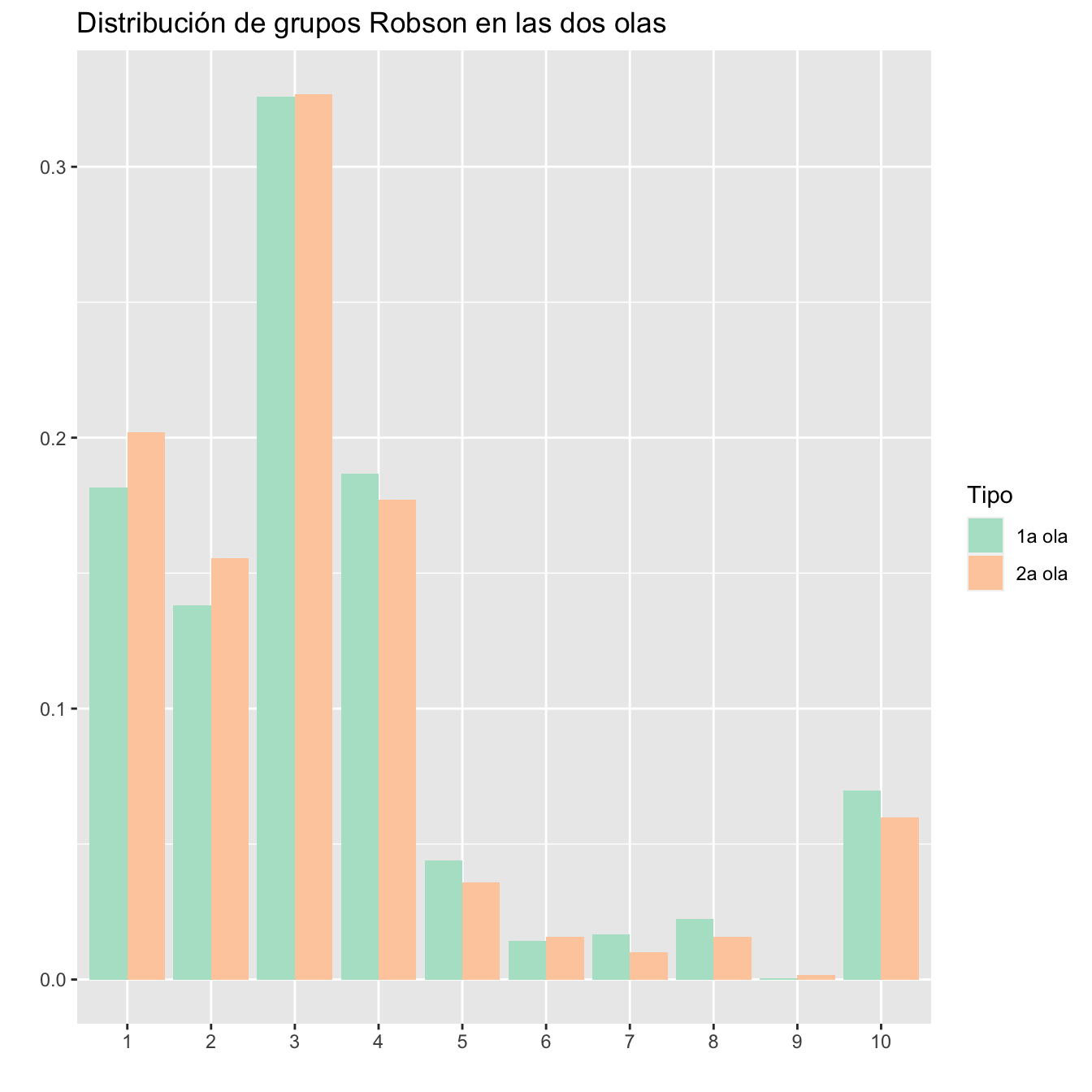
Figura 10.1:
Diferencia en la distribución de grupos Robson en las dos olas: Test \(\chi^2\) de Montecarlo (hay muy pocas gestantes del grupo 9), p-valor 0.245. No hay evidencia de diferencia en la distribución de los grupos en las dos olas.
10.1.1 Infectadas
TRCa=table(Casos$Robson,Casos$Cesárea)

DFTRCa=data.frame(Robson=c(1:10,"Pérdidas"),Gestantes=as.vector(table(Casos$Robson)[c(2:11,1)]),Cesáreas=TRCa[c(2:11,1),2], Porcentaje=round(100*prop.table(TRCa,margin=1)[c(2:11,1),2],2))
row.names(DFTRCa)=c()

DFTRCa %>%
  kbl() %>%
kable_styling()| Robson | Gestantes | Cesáreas | Porcentaje |
|---|---|---|---|
| 1 | 258 | 28 | 10.85 |
| 2 | 250 | 84 | 33.60 |
| 3 | 509 | 30 | 5.89 |
| 4 | 332 | 72 | 21.69 |
| 5 | 77 | 77 | 100.00 |
| 6 | 31 | 31 | 100.00 |
| 7 | 26 | 26 | 100.00 |
| 8 | 31 | 19 | 61.29 |
| 9 | 2 | 2 | 100.00 |
| 10 | 139 | 67 | 48.20 |
| Pérdidas | 13 | 0 | 0.00 |
Tipo=factor(rep(c("Cesárea","No cesárea"), each=10))
Grupo=factor(rep(1:10 , 2))
valor=as.vector(TRCa[c(2:11),2:1])
data=data.frame(Grupo,Tipo,valor)

ggplot(data, aes(fill=Tipo, y=valor, x=Grupo)) +
  geom_bar(position="stack", stat="identity")+
  ylab("")+
  xlab("")+
  ggtitle("Cesáreas en grupos Robson de infectadas")+
scale_fill_brewer(palette = "Pastel1") 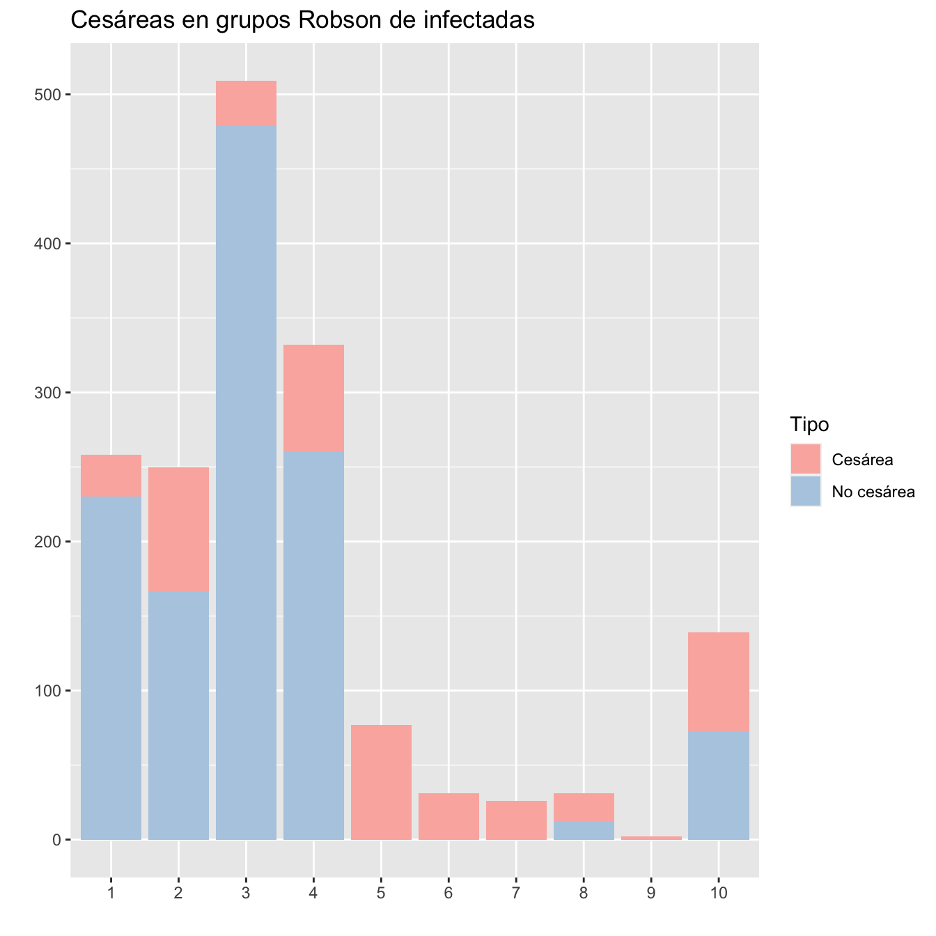
Figura 10.2:
10.1.2 No infectadas
TRCo=table(Controls$Robson,Controls$Cesárea)
DFTRCo=data.frame(Robson=c(1:10,"Pérdidas"),Gestantes=as.vector(table(Controls$Robson)[c(2:11,1)]),Cesáreas=TRCo[c(2:11,1),2], Porcentaje=round(100*prop.table(TRCo,margin=1)[c(2:11,1),2],2))
row.names(DFTRCo)=c()
DFTRCo %>%
  kbl() %>%
kable_styling()| Robson | Gestantes | Cesáreas | Porcentaje |
|---|---|---|---|
| 1 | 357 | 43 | 12.04 |
| 2 | 220 | 70 | 31.82 |
| 3 | 551 | 32 | 5.81 |
| 4 | 263 | 43 | 16.35 |
| 5 | 56 | 56 | 100.00 |
| 6 | 17 | 16 | 94.12 |
| 7 | 20 | 20 | 100.00 |
| 8 | 34 | 17 | 50.00 |
| 9 | 1 | 1 | 100.00 |
| 10 | 76 | 26 | 34.21 |
| Pérdidas | 12 | 4 | 33.33 |
Tipo=factor(rep(c("Cesárea","No cesárea"), each=10))
Grupo=factor(rep(1:10 , 2))
valor=as.vector(TRCo[c(2:11),2:1])
data=data.frame(Grupo,Tipo,valor)

ggplot(data, aes(fill=Tipo, y=valor, x=Grupo)) +
  geom_bar(position="stack", stat="identity")+
  ylab("")+
  xlab("")+
  ggtitle("Cesáreas en grupos Robson de no infectadas")+
scale_fill_brewer(palette = "Pastel1") 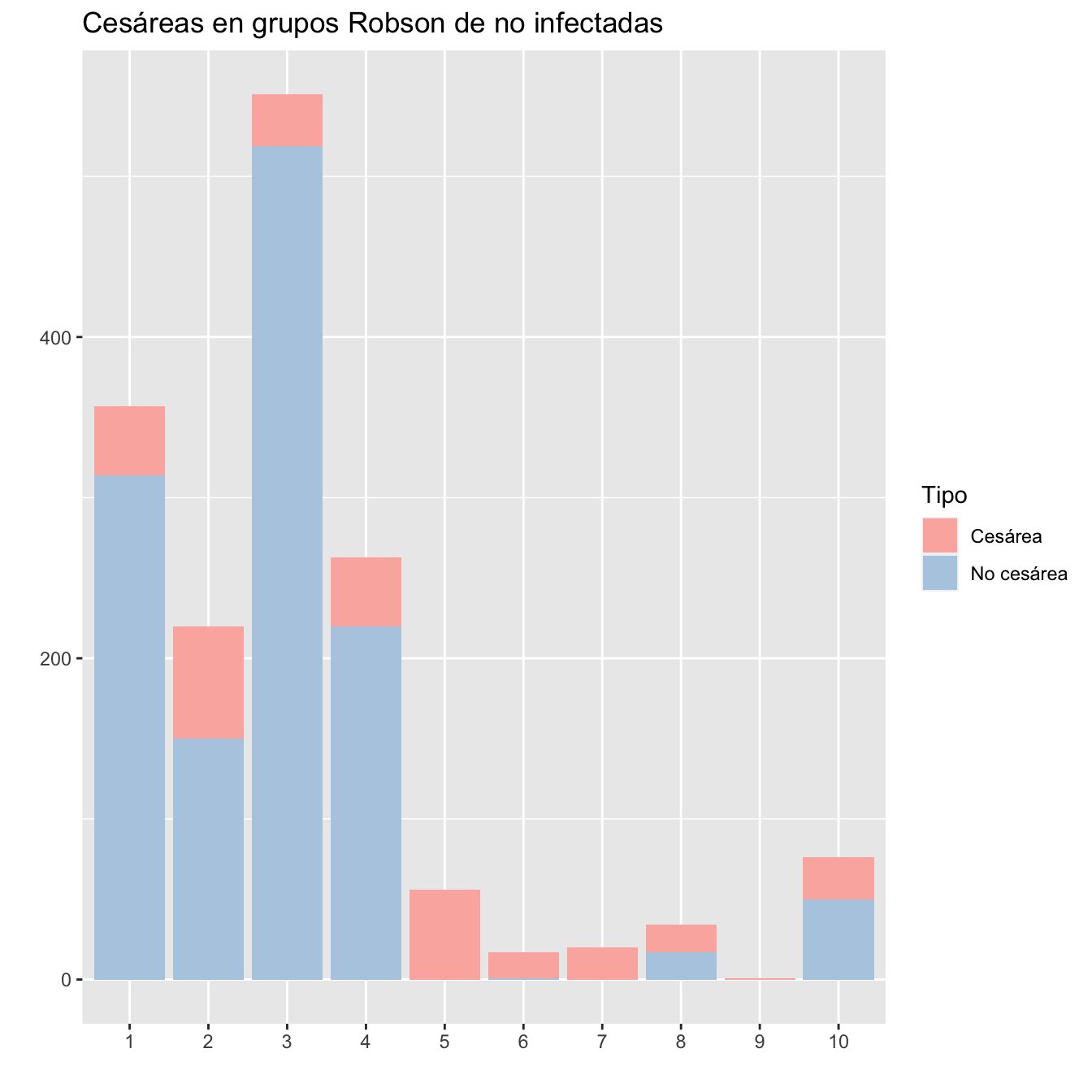
Figura 10.3:
10.1.3 Diferencias?
Diferencia en la distribución de grupos Robson entre casos y controles: Test \(\chi^2\) de Montecarlo (hay muy pocas gestantes del grupo 9), p-valor \(5\times 10^{-4}\).
Qué grupos tienen proporciones de cesáreas en infectadas o no infectadas significativamente diferentes? Ninguno:
| Grupo Robson | Casos global | Cesáreas | Porcentaje | Controles global | Cesáreas | Porcentaje | OR | p-valor test de Fisher |
|---|---|---|---|---|---|---|---|---|
| 1 | 258 | 28 | 10.85 | 357 | 43 | 12.04 | 0.89 | 0.702 |
| 2 | 250 | 84 | 33.60 | 220 | 70 | 31.82 | 1.08 | 0.695 |
| 3 | 509 | 30 | 5.89 | 551 | 32 | 5.81 | 1.02 | 1.000 |
| 4 | 332 | 72 | 21.69 | 263 | 43 | 16.35 | 1.42 | 0.117 |
| 5 | 77 | 77 | 100.00 | 56 | 56 | 100.00 | 0.00 | 1.000 |
| 6 | 31 | 31 | 100.00 | 17 | 16 | 94.12 | Inf | 0.354 |
| 7 | 26 | 26 | 100.00 | 20 | 20 | 100.00 | 0.00 | 1.000 |
| 8 | 31 | 19 | 61.29 | 34 | 17 | 50.00 | 1.57 | 0.456 |
| 9 | 2 | 2 | 100.00 | 1 | 1 | 100.00 | 0.00 | 1.000 |
| 10 | 139 | 67 | 48.20 | 76 | 26 | 34.21 | 1.78 | 0.061 |
10.1.4 Grupos sintomáticos
TCaAsin=table(Casos$Robson[Casos$SINTOMAS_CAT==1],Casos$Cesárea[Casos$SINTOMAS_CAT==1])[2:11,2:1]
TCaSL=table(Casos$Robson[Casos$SINTOMAS_CAT==2],Casos$Cesárea[Casos$SINTOMAS_CAT==2])[2:11,2:1]
TCaNeu=table(Casos$Robson[Casos$SINTOMAS_CAT==3],Casos$Cesárea[Casos$SINTOMAS_CAT==3])[2:11,2:1]
dades=data.frame(1:10,
rowSums(TCaAsin),TCaAsin[,1],round(100*prop.table(TCaAsin,margin=1)[,1],2),
rowSums(TCaSL),TCaSL[,1],round(100*prop.table(TCaSL,margin=1)[,1],2),
rowSums(TCaNeu),TCaNeu[,1],round(100*prop.table(TCaNeu,margin=1)[,1],2))
      names(dades)=c("Grupo Robson", "Inf. Asintomática", "Cesáreas", "Porcentaje",
                     "Inf. leve", "Cesáreas", "Porcentaje",
                     "Inf. grave", "Cesáreas", "Porcentaje")
dades %>%
  kbl() %>%
  kable_styling()%>%
scroll_box(width="100%", box_css="border: 0px;")| Grupo Robson | Inf. Asintomática | Cesáreas | Porcentaje | Inf. leve | Cesáreas | Porcentaje | Inf. grave | Cesáreas | Porcentaje |
|---|---|---|---|---|---|---|---|---|---|
| 1 | 125 | 17 | 13.60 | 112 | 8 | 7.14 | 21 | 3 | 14.29 |
| 2 | 120 | 43 | 35.83 | 91 | 26 | 28.57 | 39 | 15 | 38.46 |
| 3 | 252 | 14 | 5.56 | 181 | 10 | 5.52 | 76 | 6 | 7.89 |
| 4 | 132 | 24 | 18.18 | 135 | 29 | 21.48 | 65 | 19 | 29.23 |
| 5 | 30 | 30 | 100.00 | 31 | 31 | 100.00 | 16 | 16 | 100.00 |
| 6 | 13 | 13 | 100.00 | 14 | 14 | 100.00 | 4 | 4 | 100.00 |
| 7 | 9 | 9 | 100.00 | 12 | 12 | 100.00 | 5 | 5 | 100.00 |
| 8 | 8 | 5 | 62.50 | 17 | 9 | 52.94 | 6 | 5 | 83.33 |
| 9 | 1 | 1 | 100.00 | 1 | 1 | 100.00 | 0 | 0 | |
| 10 | 46 | 16 | 34.78 | 47 | 20 | 42.55 | 46 | 31 | 67.39 |
En la lista que sigue, los p-valores son los del contraste si las proporciones de cesáreas en los grupos 1,2,3,4,8 y 10 son las mismas o no en los dos grupos sintomáticos comparados:
pp=c()
EE=dades[c(1:4,8,10),c(2,3,5,6,8,9)]
pp[1]=Prop.trend.test(EE[,2],EE[,1])
pp[2]=Prop.trend.test(EE[,2],EE[,1])
pp[3]=Prop.trend.test(EE[,4],EE[,3])- Asintomática contra Leve: \(2\times 10^{-9}\)
- Asintomática contra Grave: \(2\times 10^{-9}\)
- Leve contra Grave: \(8\times 10^{-9}\)
Qué pasa si agrupamos Asintomática+Leve contra Grave? Hay diferencia en la 10
Casos$SintGrave=NA
Casos$SintGrave[Casos$SINTOMAS_CAT==1 |Casos$SINTOMAS_CAT==2]=0
Casos$SintGrave[Casos$SINTOMAS_CAT==3]=1

TCaSL=table(Casos$Robson[Casos$SintGrave==0],Casos$Cesárea[Casos$SintGrave==0])
TCaSG=table(Casos$Robson[Casos$SintGrave==1],Casos$Cesárea[Casos$SintGrave==1])

EE1=t(TCaSL)[2:1,2:11]
EE2=t(TCaSG)[2:1,2:11]
OR=rep(0,10)
pp=rep(0,10)
for (i in 1:10){
FT=fisher.test(cbind(EE1[,i],EE2[,i]))
OR[i]=FT$estimate
pp[i]=FT$p.value       }

dt=data.frame(1:10,colSums(EE1),EE1[1,],round(100*prop.table(EE1,margin=2)[1,],2),colSums(EE2),EE2[1,],round(100*prop.table(EE2,margin=2)[1,],2),round(OR,2),round(pp,3))
names(dt)=c("Grupo Robson", "Inf. Asintomática o leve", "Cesáreas", "Porcentaje",  "Inf. Grave", "Cesáreas", "Porcentaje","OR","p-valor test de Fisher")
dt %>%
  kbl() %>%
  kable_styling()%>%
scroll_box(width="100%", box_css="border: 0px;")| Grupo Robson | Inf. Asintomática o leve | Cesáreas | Porcentaje | Inf. Grave | Cesáreas | Porcentaje | OR | p-valor test de Fisher |
|---|---|---|---|---|---|---|---|---|
| 1 | 237 | 25 | 10.55 | 21 | 3 | 14.29 | 0.71 | 0.485 |
| 2 | 211 | 69 | 32.70 | 39 | 15 | 38.46 | 0.78 | 0.580 |
| 3 | 433 | 24 | 5.54 | 76 | 6 | 7.89 | 0.69 | 0.428 |
| 4 | 267 | 53 | 19.85 | 65 | 19 | 29.23 | 0.60 | 0.130 |
| 5 | 61 | 61 | 100.00 | 16 | 16 | 100.00 | 0.00 | 1.000 |
| 6 | 27 | 27 | 100.00 | 4 | 4 | 100.00 | 0.00 | 1.000 |
| 7 | 21 | 21 | 100.00 | 5 | 5 | 100.00 | 0.00 | 1.000 |
| 8 | 25 | 14 | 56.00 | 6 | 5 | 83.33 | 0.26 | 0.363 |
| 9 | 2 | 2 | 100.00 | 0 | 0 | 0.00 | 1.000 | |
| 10 | 93 | 36 | 38.71 | 46 | 31 | 67.39 | 0.31 | 0.002 |
10.2 1a ola
10.2.1 Global
TRC1w=table(c(Casos1w$Robson,Controls1w$Robson),c(Casos1w$Cesárea,Controls1w$Cesárea))
DFTRC1w=data.frame(Robson=c(1:10,"Pérdidas"),Gestantes=as.vector(table(c(Casos1w$Robson,Controls1w$Robson))[c(2:11,1)]),Cesáreas=TRC1w[c(2:11,1),2], Porcentaje=round(100*prop.table(TRC1w,margin=1)[c(2:11,1),2],2))
row.names(DFTRC1w)=c()

DFTRC1w %>%
  kbl() %>%
kable_styling()| Robson | Gestantes | Cesáreas | Porcentaje |
|---|---|---|---|
| 1 | 372 | 45 | 12.10 |
| 2 | 283 | 87 | 30.74 |
| 3 | 667 | 38 | 5.70 |
| 4 | 382 | 82 | 21.47 |
| 5 | 90 | 90 | 100.00 |
| 6 | 29 | 29 | 100.00 |
| 7 | 34 | 34 | 100.00 |
| 8 | 46 | 23 | 50.00 |
| 9 | 1 | 1 | 100.00 |
| 10 | 143 | 63 | 44.06 |
| Pérdidas | 21 | 4 | 19.05 |
Tipo=factor(rep(c("Cesárea","No cesárea"), each=10))
Grupo=factor(rep(1:10 , 2))
valor=as.vector(TRC1w[c(2:11),2:1])
data=data.frame(Grupo,Tipo,valor)

ggplot(data, aes(fill=Tipo, y=valor, x=Grupo)) +
  geom_bar(position="stack", stat="identity")+
  ylab("")+
  xlab("")+
  ggtitle("Cesáreas en grupos Robson en la 1a ola")+
scale_fill_brewer(palette = "Pastel1") 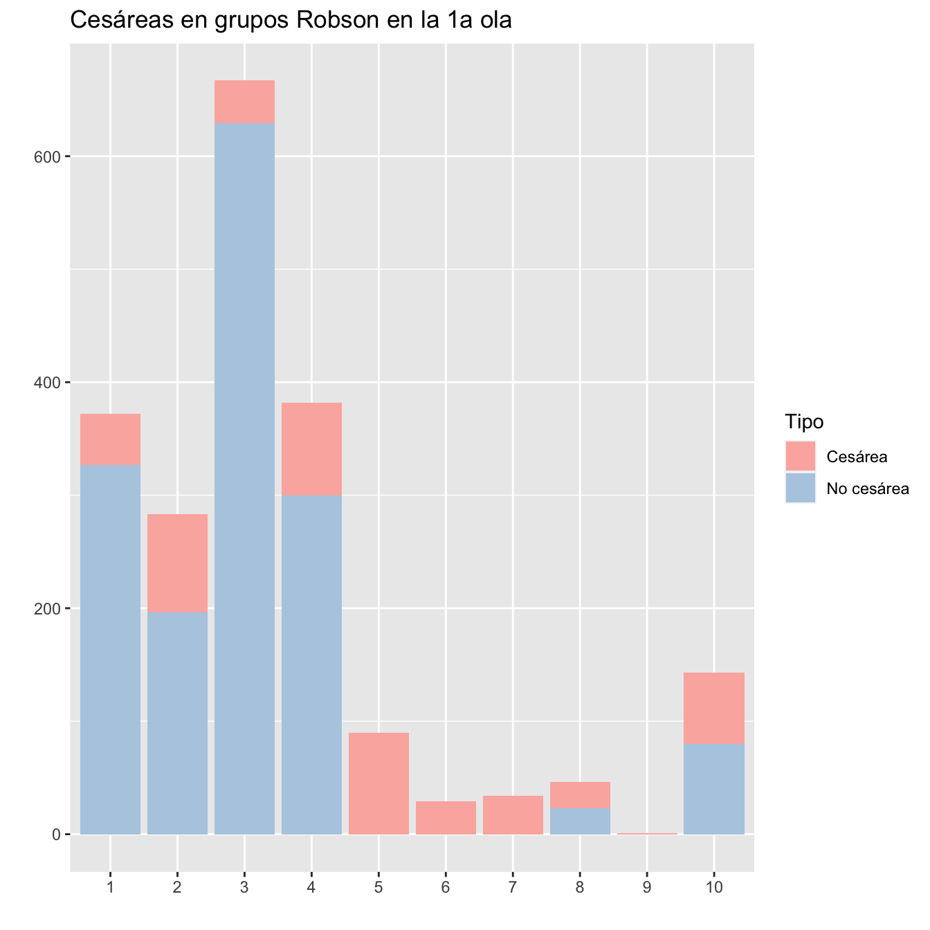
Figura 10.4:
10.2.2 Infectadas
TRCa1w=table(Casos1w$Robson,Casos1w$Cesárea)
DFTRCa1w=data.frame(Robson=c(1:10,"Pérdidas"),Gestantes=as.vector(table(Casos1w$Robson)[c(2:11,1)]),Cesáreas=TRCa1w[c(2:11,1),2], Porcentaje=round(100*prop.table(TRCa1w,margin=1)[c(2:11,1),2],2))
row.names(DFTRCa1w)=c()

DFTRCa1w %>%
  kbl() %>%
kable_styling()| Robson | Gestantes | Cesáreas | Porcentaje |
|---|---|---|---|
| 1 | 128 | 16 | 12.50 |
| 2 | 125 | 40 | 32.00 |
| 3 | 253 | 16 | 6.32 |
| 4 | 176 | 44 | 25.00 |
| 5 | 44 | 44 | 100.00 |
| 6 | 19 | 19 | 100.00 |
| 7 | 17 | 17 | 100.00 |
| 8 | 18 | 10 | 55.56 |
| 9 | 0 | 0 | |
| 10 | 86 | 43 | 50.00 |
| Pérdidas | 11 | 0 | 0.00 |
Tipo=factor(rep(c("Cesárea","No cesárea"), each=10))
Grupo=factor(rep(1:10 , 2))
valor=as.vector(TRCa1w[c(2:11),2:1])
data=data.frame(Grupo,Tipo,valor)

ggplot(data, aes(fill=Tipo, y=valor, x=Grupo)) +
  geom_bar(position="stack", stat="identity")+
  ylab("")+
  xlab("")+
  ggtitle("Cesáreas en grupos Robson en las infectadas de la 1a ola")+
scale_fill_brewer(palette = "Pastel1") 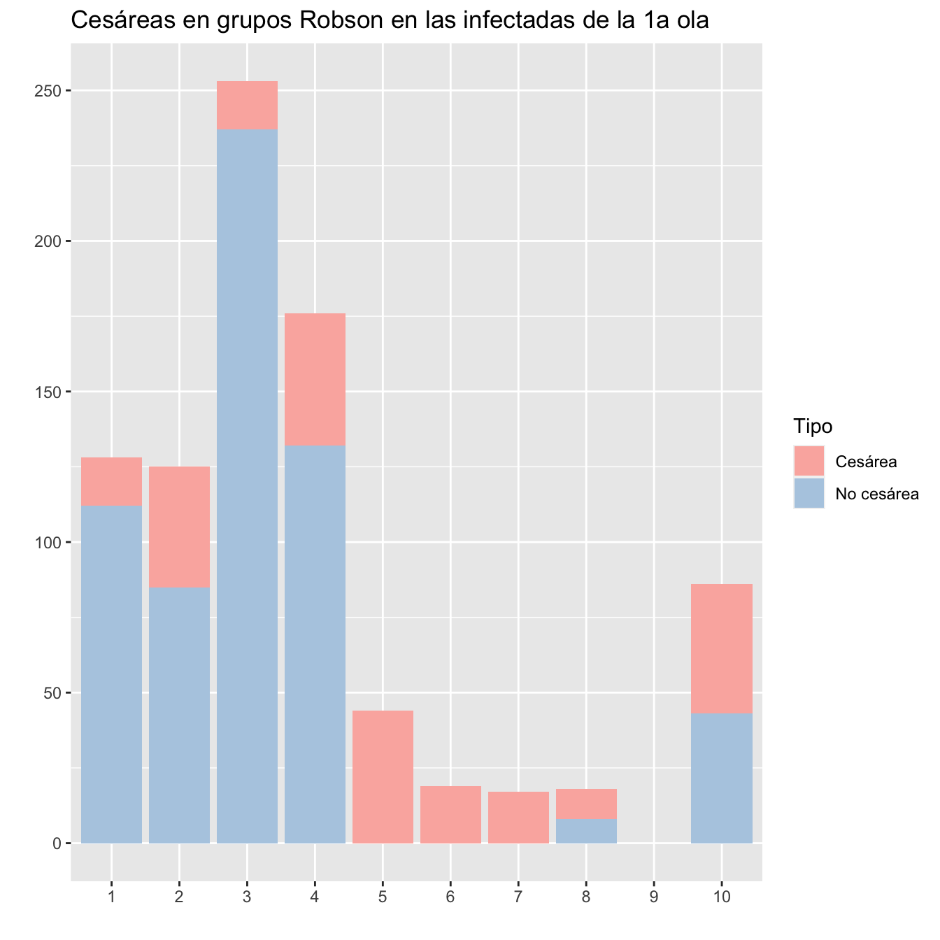
Figura 10.5:
10.2.3 No infectadas
TRCo1w=table(Controls1w$Robson,Controls1w$Cesárea)
DFTRCo1w=data.frame(Robson=c(1:10,"Pérdidas"),Gestantes=as.vector(table(Controls1w$Robson)[c(2:11,1)]),Cesáreas=TRCo1w[c(2:11,1),2], Porcentaje=round(100*prop.table(TRCo1w,margin=1)[c(2:11,1),2],2))
row.names(DFTRCo1w)=c()

DFTRCo1w %>%
  kbl() %>%
kable_styling()| Robson | Gestantes | Cesáreas | Porcentaje |
|---|---|---|---|
| 1 | 244 | 29 | 11.89 |
| 2 | 158 | 47 | 29.75 |
| 3 | 414 | 22 | 5.31 |
| 4 | 206 | 38 | 18.45 |
| 5 | 46 | 46 | 100.00 |
| 6 | 10 | 10 | 100.00 |
| 7 | 17 | 17 | 100.00 |
| 8 | 28 | 13 | 46.43 |
| 9 | 1 | 1 | 100.00 |
| 10 | 57 | 20 | 35.09 |
| Pérdidas | 10 | 4 | 40.00 |
Tipo=factor(rep(c("Cesárea","No cesárea"), each=10))
Grupo=factor(rep(1:10 , 2))
valor=as.vector(TRCo1w[c(2:11),2:1])
data=data.frame(Grupo,Tipo,valor)

ggplot(data, aes(fill=Tipo, y=valor, x=Grupo)) +
  geom_bar(position="stack", stat="identity")+
  ylab("")+
  xlab("")+
  ggtitle("Cesáreas en grupos Robson en las no infectadas de la 1a ola")+
scale_fill_brewer(palette = "Pastel1") 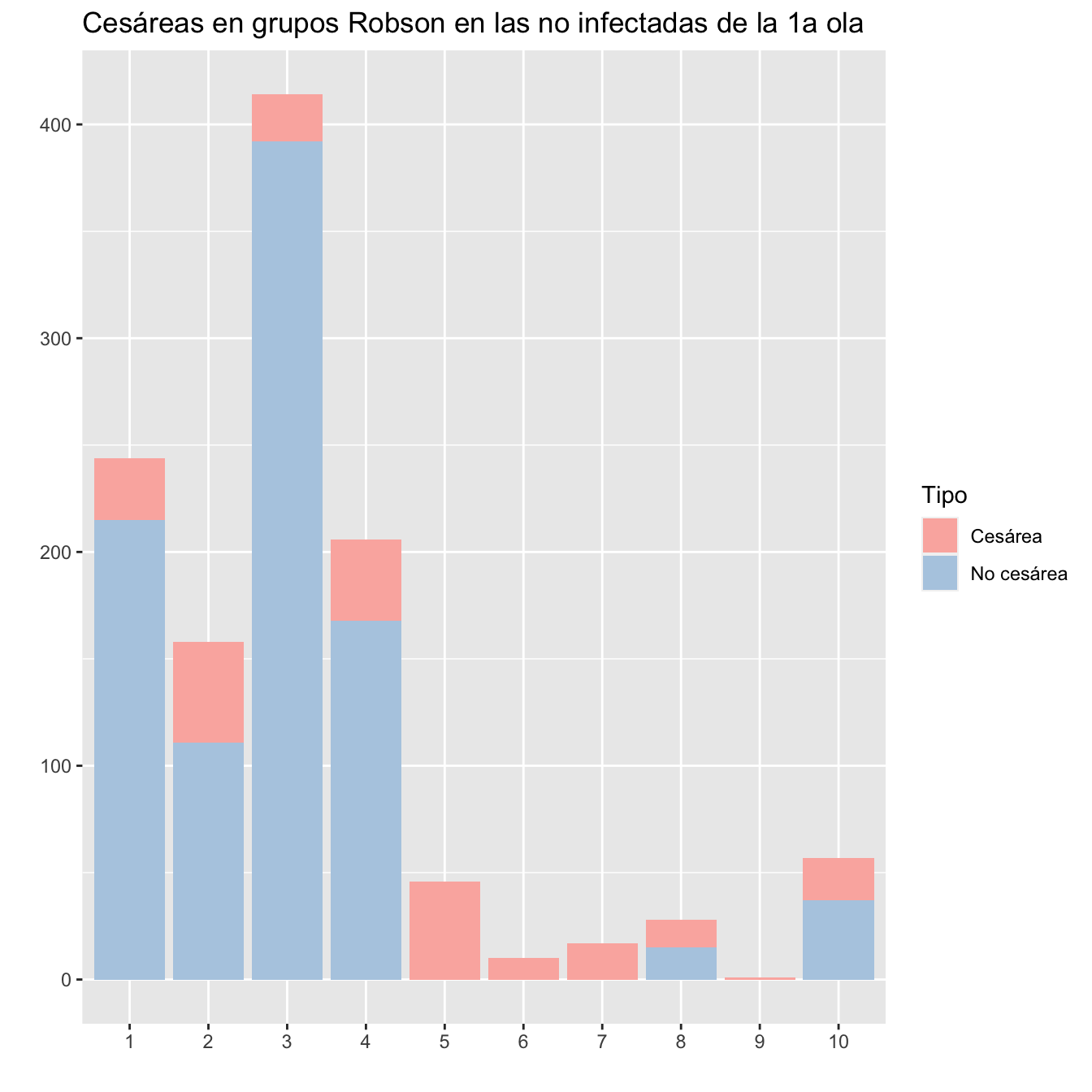
Figura 10.6:
10.2.4 Diferencias?
Qué grupos tienen proporciones de cesáreas significativamente diferentes entre infectadas y no infectadas? Ninguno:
| Grupo Robson | Casos global | Cesáreas | Porcentaje | Controles global | Cesáreas | Porcentaje | OR | p-valor test de Fisher |
|---|---|---|---|---|---|---|---|---|
| 1 | 128 | 16 | 12.50 | 244 | 29 | 11.89 | 1.06 | 0.868 |
| 2 | 125 | 40 | 32.00 | 158 | 47 | 29.75 | 1.11 | 0.699 |
| 3 | 253 | 16 | 6.32 | 414 | 22 | 5.31 | 1.20 | 0.608 |
| 4 | 176 | 44 | 25.00 | 206 | 38 | 18.45 | 1.47 | 0.134 |
| 5 | 44 | 44 | 100.00 | 46 | 46 | 100.00 | 0.00 | 1.000 |
| 6 | 19 | 19 | 100.00 | 10 | 10 | 100.00 | 0.00 | 1.000 |
| 7 | 17 | 17 | 100.00 | 17 | 17 | 100.00 | 0.00 | 1.000 |
| 8 | 18 | 10 | 55.56 | 28 | 13 | 46.43 | 1.43 | 0.763 |
| 9 | 0 | 0 | 1 | 1 | 100.00 | 0.00 | 1.000 | |
| 10 | 86 | 43 | 50.00 | 57 | 20 | 35.09 | 1.84 | 0.088 |
10.3 2a ola
10.3.1 Global
TRC2w=table(c(Casos2w$Robson,Controls2w$Robson),c(Casos2w$Cesárea,Controls2w$Cesárea))
DFTRC2w=data.frame(Robson=c(1:10,"Pérdidas"),Gestantes=as.vector(table(c(Casos2w$Robson,Controls2w$Robson))[c(2:11,1)]),Cesáreas=TRC2w[c(2:11,1),2], Porcentaje=round(100*prop.table(TRC2w,margin=1)[c(2:11,1),2],2))
row.names(DFTRC2w)=c()

DFTRC2w %>%
  kbl() %>%
kable_styling()| Robson | Gestantes | Cesáreas | Porcentaje |
|---|---|---|---|
| 1 | 243 | 26 | 10.70 |
| 2 | 187 | 67 | 35.83 |
| 3 | 393 | 24 | 6.11 |
| 4 | 213 | 33 | 15.49 |
| 5 | 43 | 43 | 100.00 |
| 6 | 19 | 18 | 94.74 |
| 7 | 12 | 12 | 100.00 |
| 8 | 19 | 13 | 68.42 |
| 9 | 2 | 2 | 100.00 |
| 10 | 72 | 30 | 41.67 |
| Pérdidas | 4 | 0 | 0.00 |
Tipo=factor(rep(c("Cesárea","No cesárea"), each=10))
Grupo=factor(rep(1:10 , 2))
valor=as.vector(TRC2w[c(2:11),2:1])
data=data.frame(Grupo,Tipo,valor)

ggplot(data, aes(fill=Tipo, y=valor, x=Grupo)) +
  geom_bar(position="stack", stat="identity")+
  ylab("")+
  xlab("")+
  ggtitle("Cesáreas en grupos Robson en la 2a ola")+
scale_fill_brewer(palette = "Pastel1") 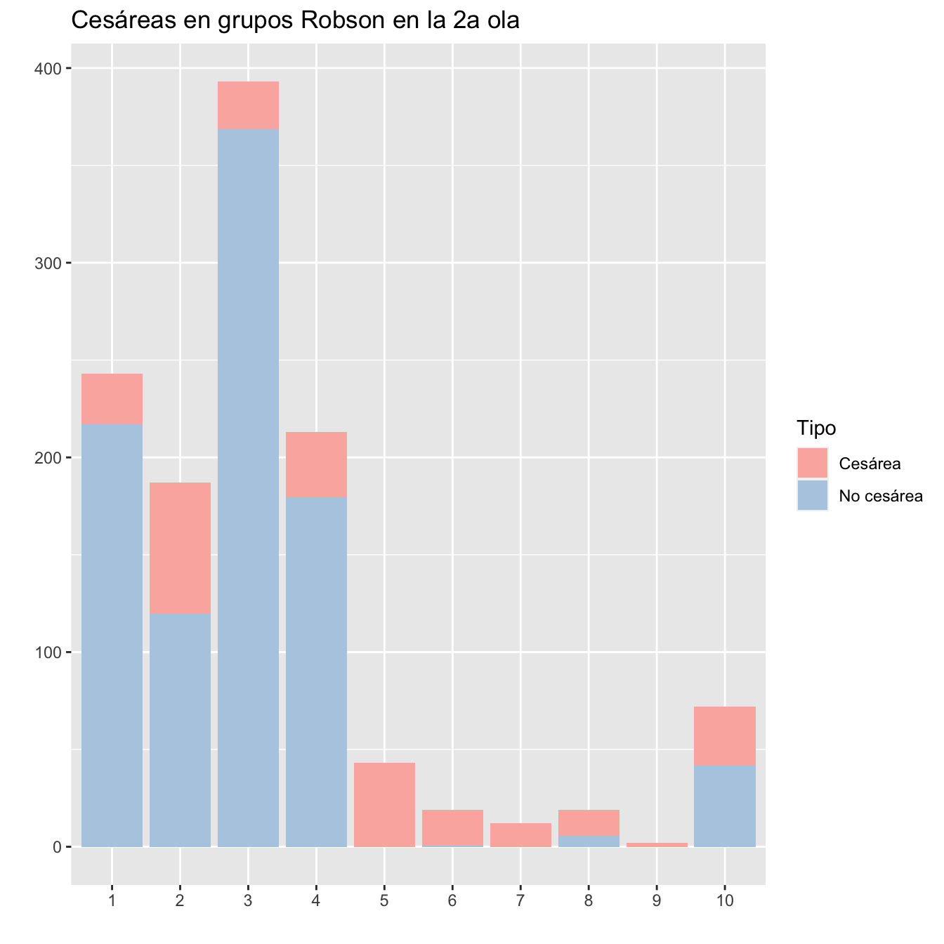
Figura 10.7:
10.3.2 Infectadas
TRCa2w=table(Casos2w$Robson,Casos2w$Cesárea)
DFTRCa2w=data.frame(Robson=c(1:10,"Pérdidas"),Gestantes=as.vector(table(Casos2w$Robson)[c(2:11,1)]),Cesáreas=TRCa2w[c(2:11,1),2], Porcentaje=round(100*prop.table(TRCa2w,margin=1)[c(2:11,1),2],2))
row.names(DFTRCa2w)=c()

DFTRCa2w %>%
  kbl() %>%
kable_styling()| Robson | Gestantes | Cesáreas | Porcentaje |
|---|---|---|---|
| 1 | 130 | 12 | 9.23 |
| 2 | 125 | 44 | 35.20 |
| 3 | 256 | 14 | 5.47 |
| 4 | 156 | 28 | 17.95 |
| 5 | 33 | 33 | 100.00 |
| 6 | 12 | 12 | 100.00 |
| 7 | 9 | 9 | 100.00 |
| 8 | 13 | 9 | 69.23 |
| 9 | 2 | 2 | 100.00 |
| 10 | 53 | 24 | 45.28 |
| Pérdidas | 2 | 0 | 0.00 |
Tipo=factor(rep(c("Cesárea","No cesárea"), each=10))
Grupo=factor(rep(1:10 , 2))
valor=as.vector(TRCa2w[c(2:11),2:1])
data=data.frame(Grupo,Tipo,valor)

ggplot(data, aes(fill=Tipo, y=valor, x=Grupo)) +
  geom_bar(position="stack", stat="identity")+
  ylab("")+
  xlab("")+
  ggtitle("Cesáreas en grupos Robson en las infectadas de la 2a ola")+
scale_fill_brewer(palette = "Pastel1") 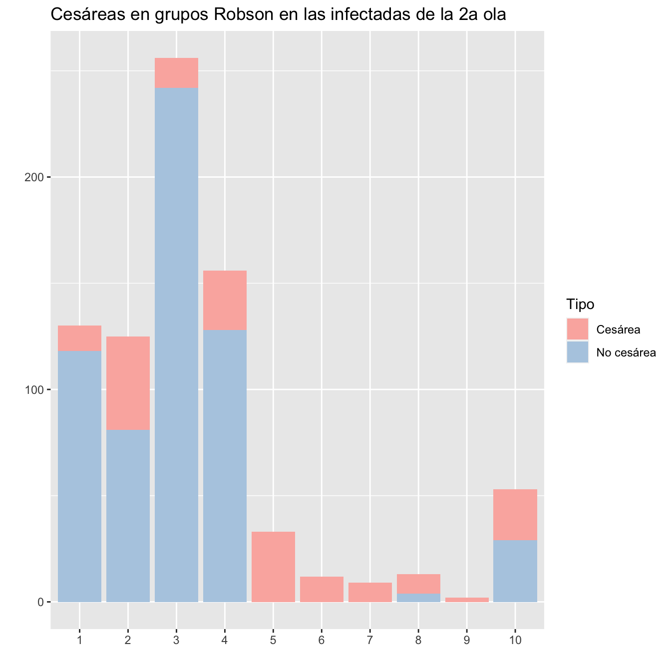
Figura 10.8:
10.3.3 No infectadas
TRCo2w=table(Controls2w$Robson,Controls2w$Cesárea)
DFTRCo2w=data.frame(Robson=c(1:10,"Pérdidas"),Gestantes=as.vector(table(Controls2w$Robson)[c(2:11,1)]),Cesáreas=TRCo2w[c(2:11,1),2], Porcentaje=round(100*prop.table(TRCo2w,margin=1)[c(2:11,1),2],2))
row.names(DFTRCo2w)=c()

DFTRCo2w %>%
  kbl() %>%
kable_styling()| Robson | Gestantes | Cesáreas | Porcentaje |
|---|---|---|---|
| 1 | 113 | 14 | 12.39 |
| 2 | 62 | 23 | 37.10 |
| 3 | 137 | 10 | 7.30 |
| 4 | 57 | 5 | 8.77 |
| 5 | 10 | 10 | 100.00 |
| 6 | 7 | 6 | 85.71 |
| 7 | 3 | 3 | 100.00 |
| 8 | 6 | 4 | 66.67 |
| 9 | 0 | 0 | |
| 10 | 19 | 6 | 31.58 |
| Pérdidas | 2 | 0 | 0.00 |
Tipo=factor(rep(c("Cesárea","No cesárea"), each=10))
Grupo=factor(rep(1:10 , 2))
valor=as.vector(TRCo2w[c(2:11),2:1])
data=data.frame(Grupo,Tipo,valor)

ggplot(data, aes(fill=Tipo, y=valor, x=Grupo)) +
  geom_bar(position="stack", stat="identity")+
  ylab("")+
  xlab("")+
  ggtitle("Cesáreas en grupos Robson en las no infectadas de la 2a ola")+
scale_fill_brewer(palette = "Pastel1") 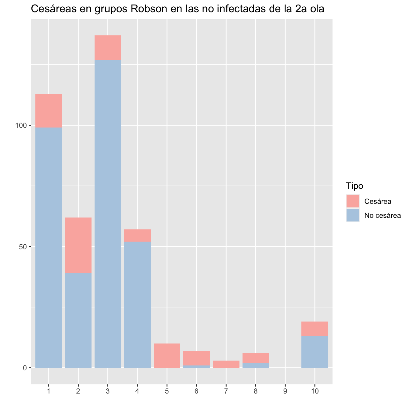
Figura 10.9:
10.3.4 Diferencias?
Qué grupos tienen proporciones de cesáreas significativamente diferentes? Ninguno:
| Grupo Robson | Casos 2a ola | Cesáreas | Porcentaje | Controles 2a ola | Cesáreas | Porcentaje | OR | p-valor test de Fisher |
|---|---|---|---|---|---|---|---|---|
| 1 | 130 | 12 | 9.23 | 113 | 14 | 12.39 | 0.72 | 0.533 |
| 2 | 125 | 44 | 35.20 | 62 | 23 | 37.10 | 0.92 | 0.872 |
| 3 | 256 | 14 | 5.47 | 137 | 10 | 7.30 | 0.74 | 0.510 |
| 4 | 156 | 28 | 17.95 | 57 | 5 | 8.77 | 2.27 | 0.134 |
| 5 | 33 | 33 | 100.00 | 10 | 10 | 100.00 | 0.00 | 1.000 |
| 6 | 12 | 12 | 100.00 | 7 | 6 | 85.71 | Inf | 0.368 |
| 7 | 9 | 9 | 100.00 | 3 | 3 | 100.00 | 0.00 | 1.000 |
| 8 | 13 | 9 | 69.23 | 6 | 4 | 66.67 | 1.12 | 1.000 |
| 9 | 2 | 2 | 100.00 | 0 | 0 | 0.00 | 1.000 | |
| 10 | 53 | 24 | 45.28 | 19 | 6 | 31.58 | 1.78 | 0.417 |
10.4 Contrastes entre olas
10.4.1 En el global
Qué grupos tienen proporciones de cesáreas significativamente diferentes en las dos olas? Ninguno:
EE1=t(TRC1w)[2:1,2:11]
EE2=t(TRC2w)[2:1,2:11]
OR=rep(0,10)
pp=rep(0,10)
for (i in 1:10){
FT=fisher.test(cbind(EE1[,i],EE2[,i]))
OR[i]=FT$estimate
pp[i]=FT$p.value       }

dt=data.frame(1:10,colSums(EE1),EE1[1,],round(100*prop.table(EE1,margin=2)[1,],2),colSums(EE2),EE2[1,],round(100*prop.table(EE2,margin=2)[1,],2),round(OR,2),round(pp,3))
names(dt)=c("Grupo Robson", "1a ola", "Cesáreas", "Porcentaje",  "2a ola", "Cesáreas", "Porcentaje","OR","p-valor test de Fisher")
dt %>%
  kbl() %>%
  kable_styling()%>%
scroll_box(width="100%", box_css="border: 0px;")| Grupo Robson | 1a ola | Cesáreas | Porcentaje | 2a ola | Cesáreas | Porcentaje | OR | p-valor test de Fisher |
|---|---|---|---|---|---|---|---|---|
| 1 | 372 | 45 | 12.10 | 243 | 26 | 10.70 | 1.15 | 0.699 |
| 2 | 283 | 87 | 30.74 | 187 | 67 | 35.83 | 0.80 | 0.270 |
| 3 | 667 | 38 | 5.70 | 393 | 24 | 6.11 | 0.93 | 0.788 |
| 4 | 382 | 82 | 21.47 | 213 | 33 | 15.49 | 1.49 | 0.084 |
| 5 | 90 | 90 | 100.00 | 43 | 43 | 100.00 | 0.00 | 1.000 |
| 6 | 29 | 29 | 100.00 | 19 | 18 | 94.74 | Inf | 0.396 |
| 7 | 34 | 34 | 100.00 | 12 | 12 | 100.00 | 0.00 | 1.000 |
| 8 | 46 | 23 | 50.00 | 19 | 13 | 68.42 | 0.47 | 0.273 |
| 9 | 1 | 1 | 100.00 | 2 | 2 | 100.00 | 0.00 | 1.000 |
| 10 | 143 | 63 | 44.06 | 72 | 30 | 41.67 | 1.10 | 0.772 |
10.4.2 Entre infectadas
Qué grupos tienen proporciones de cesáreas significativamente diferentes en las infectadas en las dos olas? Ninguno:
EE1=t(TRCa1w)[2:1,2:11]
EE2=t(TRCa2w)[2:1,2:11]
OR=rep(0,10)
pp=rep(0,10)
for (i in 1:10){
FT=fisher.test(cbind(EE1[,i],EE2[,i]))
OR[i]=FT$estimate
pp[i]=FT$p.value       }

dt=data.frame(1:10,colSums(EE1),EE1[1,],round(100*prop.table(EE1,margin=2)[1,],2),colSums(EE2),EE2[1,],round(100*prop.table(EE2,margin=2)[1,],2),round(OR,2),round(pp,3))
names(dt)=c("Grupo Robson", "Inf. 1a ola", "Cesáreas", "Porcentaje",  "Inf. 2a ola", "Cesáreas", "Porcentaje","OR","p-valor test de Fisher")
dt %>%
  kbl() %>%
  kable_styling()%>%
scroll_box(width="100%", box_css="border: 0px;")| Grupo Robson | Inf. 1a ola | Cesáreas | Porcentaje | Inf. 2a ola | Cesáreas | Porcentaje | OR | p-valor test de Fisher |
|---|---|---|---|---|---|---|---|---|
| 1 | 128 | 16 | 12.50 | 130 | 12 | 9.23 | 1.40 | 0.429 |
| 2 | 125 | 40 | 32.00 | 125 | 44 | 35.20 | 0.87 | 0.688 |
| 3 | 253 | 16 | 6.32 | 256 | 14 | 5.47 | 1.17 | 0.710 |
| 4 | 176 | 44 | 25.00 | 156 | 28 | 17.95 | 1.52 | 0.142 |
| 5 | 44 | 44 | 100.00 | 33 | 33 | 100.00 | 0.00 | 1.000 |
| 6 | 19 | 19 | 100.00 | 12 | 12 | 100.00 | 0.00 | 1.000 |
| 7 | 17 | 17 | 100.00 | 9 | 9 | 100.00 | 0.00 | 1.000 |
| 8 | 18 | 10 | 55.56 | 13 | 9 | 69.23 | 0.57 | 0.484 |
| 9 | 0 | 0 | 2 | 2 | 100.00 | 0.00 | 1.000 | |
| 10 | 86 | 43 | 50.00 | 53 | 24 | 45.28 | 1.21 | 0.605 |
10.5 Grupos sintomáticos y olas
10.5.1 Global
TRCaS=table(Casos$Robson,Casos$SINTOMAS_DIAGNOSTICO)[c(2:11,1),]
pTRCaS=round(100*prop.table(table(Casos$Robson,Casos$SINTOMAS_DIAGNOSTICO),margin=1)[c(2:11,1),],2)
DFTRCaS=data.frame(
  Robson=c(1:10,"Pérdidas"),
Tot=as.vector(table(Casos$Robson)[c(2:11,1)]),
Asint=TRCaS[,1],
pAsint=pTRCaS[,1],
SL=TRCaS[,2],
pSL=pTRCaS[,2],
Neum=TRCaS[,3],
pNeum=pTRCaS[,3])
row.names(DFTRCaS)=c()
names(DFTRCaS)=c("Grupo Robson", "Total infectadas", "Asintomática", "%", "Leve", "%", "Grave", "%")

DFTRCaS %>%
  kbl() %>%
  kable_styling()%>%
scroll_box(width="100%", box_css="border: 0px;")| Grupo Robson | Total infectadas | Asintomática | % | Leve | % | Grave | % |
|---|---|---|---|---|---|---|---|
| 1 | 258 | 125 | 48.45 | 112 | 43.41 | 21 | 8.14 |
| 2 | 250 | 120 | 48.00 | 91 | 36.40 | 39 | 15.60 |
| 3 | 509 | 252 | 49.51 | 181 | 35.56 | 76 | 14.93 |
| 4 | 332 | 132 | 39.76 | 135 | 40.66 | 65 | 19.58 |
| 5 | 77 | 30 | 38.96 | 31 | 40.26 | 16 | 20.78 |
| 6 | 31 | 13 | 41.94 | 14 | 45.16 | 4 | 12.90 |
| 7 | 26 | 9 | 34.62 | 12 | 46.15 | 5 | 19.23 |
| 8 | 31 | 8 | 25.81 | 17 | 54.84 | 6 | 19.35 |
| 9 | 2 | 1 | 50.00 | 1 | 50.00 | 0 | 0.00 |
| 10 | 139 | 46 | 33.09 | 47 | 33.81 | 46 | 33.09 |
| Pérdidas | 13 | 9 | 69.23 | 2 | 15.38 | 2 | 15.38 |
Tipo=factor(rep(c("Asintomática","Leve", "Grave"), each=10))
Grupo=factor(rep(1:10 , 3))
valor=as.vector(TRCaS[1:10,])
data=data.frame(Grupo,Tipo,valor)

ggplot(data, aes(fill=Tipo, y=valor, x=Grupo)) +
  geom_bar(position="stack", stat="identity")+
  ylab("")+
  xlab("")+
  ggtitle("Grupos sintomáticos en grupos Robson en las infectadas")+
scale_fill_brewer(palette = "Dark2") 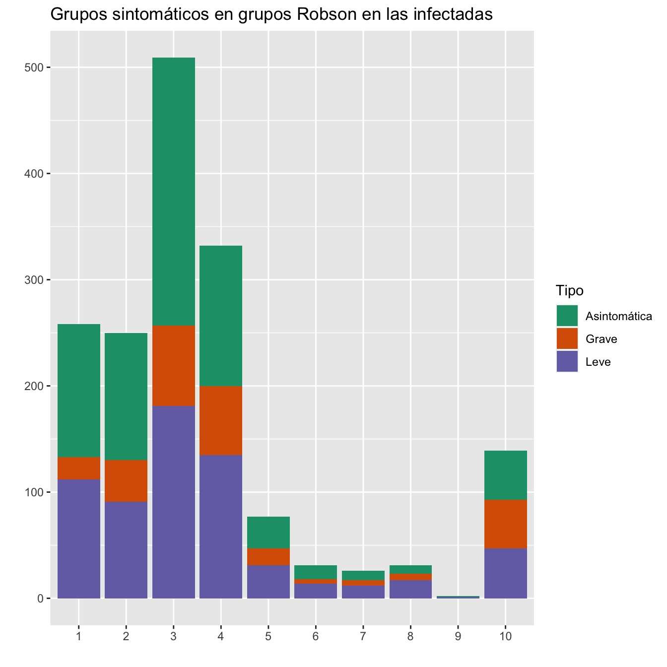
Figura 10.10:
En la tabla que sigue, para cada grupo Robson, el p-valor es del contraste \(\chi^2\) de si la distribución de los síntomas de las infectadas de ese grupo es igual o diferente de la distribución de los síntomas de las infectadas. Como ves, las distribuciones de síntomas en los grupos 1 y 10 son significativamente diferentes del global.
pp=c()
for (i in c(1:10)){
pp[i]=chisq.test(TRCaS[i,],p=prop.table(colSums(TRCaS)),simulate.p.value=TRUE,B=10000)$p.value
}
tabla=data.frame(
Robson=rep(1:10),
round(pp,4)
)
names(tabla)=c("Grupo Robson","p-valor")
row.names(tabla)=c()

tabla %>%
  kbl() %>%
  kable_styling()%>%
scroll_box(width="100%", box_css="border: 0px;")| Grupo Robson | p-valor |
|---|---|
| 1 | 0.0006 |
| 2 | 0.5724 |
| 3 | 0.0807 |
| 4 | 0.1579 |
| 5 | 0.5232 |
| 6 | 0.7208 |
| 7 | 0.5707 |
| 8 | 0.1031 |
| 9 | 1.0000 |
| 10 | 0.0001 |
10.5.2 Comparando olas
TRCa1wS=table(Casos1w$Robson,Casos1w$SINTOMAS_DIAGNOSTICO)[c(2:11,1),]
pTRCa1wS=round(100*prop.table(table(Casos1w$Robson,Casos1w$SINTOMAS_DIAGNOSTICO),margin=1)[c(2:11,1),],2)
pTRCa1wS[9,]=c(0,0,0)
TRCa2wS=table(Casos2w$Robson,Casos2w$SINTOMAS_DIAGNOSTICO)[c(2:11,1),]
pTRCa2wS=round(100*prop.table(table(Casos2w$Robson,Casos2w$SINTOMAS_DIAGNOSTICO),margin=1)[c(2:11,1),],2)
DFTRCaWS=data.frame(
  Robson=c(1:10,"Pérdidas"),
Tot1w=as.vector(table(Casos1w$Robson)[c(2:11,1)]),
Asint1w=TRCa1wS[,1],
pAsint1w=pTRCa1wS[,1],
SL1w=TRCa1wS[,2],
pSL1w=pTRCa1wS[,2],
Neum1w=TRCa1wS[,3],
pTRCa1wS[,3],
Tot2w=as.vector(table(Casos2w$Robson)[c(2:11,1)]),
Asint2w=TRCa2wS[,1],
pAsint2w=pTRCa2wS[,1],
SL2w=TRCa2wS[,2],
pSL2w=pTRCa2wS[,2],
Neum2w=TRCa2wS[,3],
pTRCa2wS[,3])
row.names(DFTRCaWS)=c()
names(DFTRCaWS)=c("Grupo Robson", "Total infectadas 1a ola", "Asintomática 1a ola", "%", "Leve 1a ola", "%", "Grave 1a ola", "%","Total infectadas 2a ola", "Asintomática 2a ola", "%", "Leve 2a ola", "%", "Grave 2a ola", "%")

DFTRCaWS %>%
  kbl() %>%
  kable_styling()%>%
scroll_box(width="100%", box_css="border: 0px;")| Grupo Robson | Total infectadas 1a ola | Asintomática 1a ola | % | Leve 1a ola | % | Grave 1a ola | % | Total infectadas 2a ola | Asintomática 2a ola | % | Leve 2a ola | % | Grave 2a ola | % |
|---|---|---|---|---|---|---|---|---|---|---|---|---|---|---|
| 1 | 128 | 58 | 45.31 | 50 | 39.06 | 20 | 15.62 | 130 | 67 | 51.54 | 62 | 47.69 | 1 | 0.77 |
| 2 | 125 | 54 | 43.20 | 44 | 35.20 | 27 | 21.60 | 125 | 66 | 52.80 | 47 | 37.60 | 12 | 9.60 |
| 3 | 253 | 120 | 47.43 | 83 | 32.81 | 50 | 19.76 | 256 | 132 | 51.56 | 98 | 38.28 | 26 | 10.16 |
| 4 | 176 | 63 | 35.80 | 63 | 35.80 | 50 | 28.41 | 156 | 69 | 44.23 | 72 | 46.15 | 15 | 9.62 |
| 5 | 44 | 15 | 34.09 | 18 | 40.91 | 11 | 25.00 | 33 | 15 | 45.45 | 13 | 39.39 | 5 | 15.15 |
| 6 | 19 | 7 | 36.84 | 9 | 47.37 | 3 | 15.79 | 12 | 6 | 50.00 | 5 | 41.67 | 1 | 8.33 |
| 7 | 17 | 4 | 23.53 | 9 | 52.94 | 4 | 23.53 | 9 | 5 | 55.56 | 3 | 33.33 | 1 | 11.11 |
| 8 | 18 | 2 | 11.11 | 12 | 66.67 | 4 | 22.22 | 13 | 6 | 46.15 | 5 | 38.46 | 2 | 15.38 |
| 9 | 0 | 0 | 0.00 | 0 | 0.00 | 0 | 0.00 | 2 | 1 | 50.00 | 1 | 50.00 | 0 | 0.00 |
| 10 | 86 | 25 | 29.07 | 26 | 30.23 | 35 | 40.70 | 53 | 21 | 39.62 | 21 | 39.62 | 11 | 20.75 |
| Pérdidas | 11 | 9 | 81.82 | 0 | 0.00 | 2 | 18.18 | 2 | 0 | 0.00 | 2 | 100.00 | 0 | 0.00 |
Tipo=factor(rep(c("Asintomática","Leve", "Grave"), each=10))
Grupo=factor(rep(1:10 , 3))
valor=as.vector(TRCa1wS[1:10,])
data=data.frame(Grupo,Tipo,valor)

ggplot(data, aes(fill=Tipo, y=valor, x=Grupo)) +
  geom_bar(position="stack", stat="identity")+
  ylab("")+
  xlab("")+
  ggtitle("Grupos sintomáticos en grupos Robson en las infectadas de la 1a ola")+
scale_fill_brewer(palette = "Dark2") 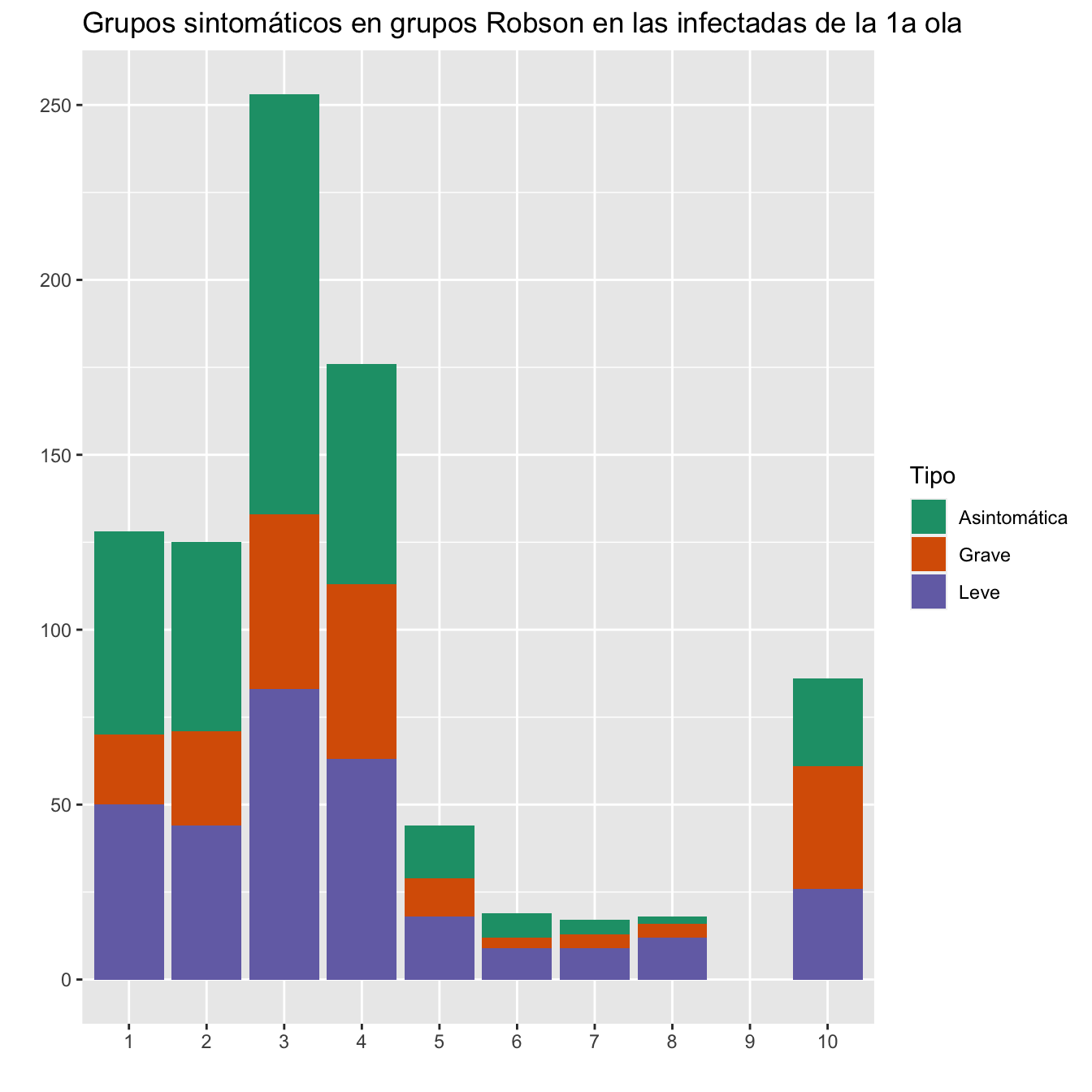
Figura 10.11:
Tipo=ordered(rep(c("Asintomática","Leve", "Grave"), each=10),levels=c("Asintomática","Leve", "Grave"))
Grupo=factor(rep(1:10 , 3))
valor=as.vector(TRCa2wS[1:10,])
data=data.frame(Grupo,Tipo,valor)

ggplot(data, aes(fill=Tipo, y=valor, x=Grupo)) +
  geom_bar(position="stack", stat="identity")+
  ylab("")+
  xlab("")+
  ggtitle("Grupos sintomáticos en grupos Robson en las infectadas de la 2a ola")+
scale_fill_brewer(palette = "Dark2") 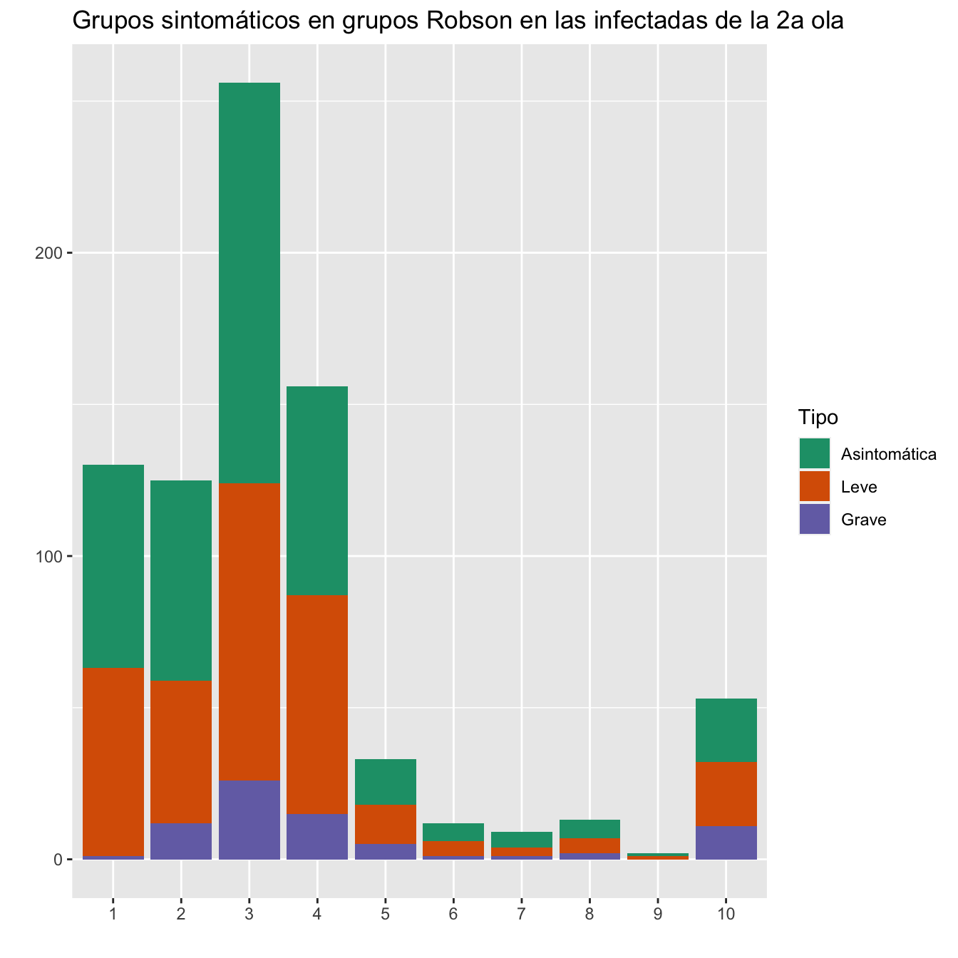
Figura 10.12:
Tipo=ordered(rep(c("Asintomática","Leve", "Grave"), 20),levels=c("Asintomática","Leve", "Grave"))
Grupo=ordered(rep(c(sort(c(paste(1:9, "\n 1a\n ola"),paste(1:9, "\n 2a\n ola")) ),"10 \n 1a\n ola", "10 \n 2a\n ola"),each=3),levels=
               c(sort(c(paste(1:9, "\n 1a\n ola"),paste(1:9, "\n 2a\n ola")) ),"10 \n 1a\n ola", "10 \n 2a\n ola"))
valor=c()
for (i in 1:10){
  valor=c(valor,pTRCa1wS[i,],  pTRCa2wS[i,])
}
data=data.frame(Grupo,Tipo,valor)

ggplot(data, aes(fill=Tipo, y=valor, x=Grupo)) +
  geom_bar(position="stack", stat="identity")+
  ylab("")+
  xlab("")+
  ggtitle("Distribuciones en grupos sintomáticos de los grupos Robson de  infectadas en ambas olas")+
scale_fill_brewer(palette = "Dark2") 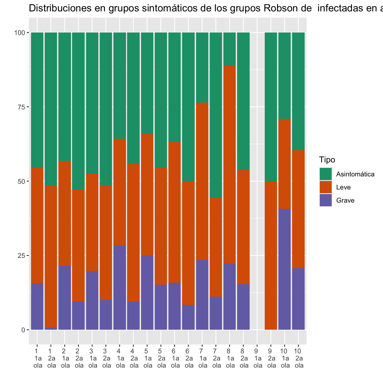
Figura 10.13:
Tipo=ordered(rep(c("Asintomática","Leve", "Grave"), 20),levels=c("Asintomática","Leve", "Grave"))
Grupo=ordered(rep(c(sort(c(paste(1:9, "\n 1a\n ola"),paste(1:9, "\n 2a\n ola")) ),"10 \n 1a\n ola", "10 \n 2a\n ola"),each=3),levels=
               c(sort(c(paste(1:9, "\n 1a\n ola"),paste(1:9, "\n 2a\n ola")) ),"10 \n 1a\n ola", "10 \n 2a\n ola"))
valor=c()
for (i in 1:10){
  valor=c(valor,TRCa1wS[i,],  TRCa2wS[i,])
}
data=data.frame(Grupo,Tipo,valor)

ggplot(data, aes(fill=Tipo, y=valor, x=Grupo)) +
  geom_bar(position="stack", stat="identity")+
  ylab("")+
  xlab("")+
  ggtitle("Frecuencias de grupos sintomáticos en los grupos Robson de  infectadas en ambas olas")+
scale_fill_brewer(palette = "Dark2") 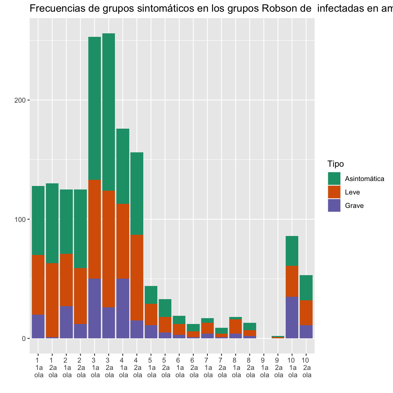
Figura 10.14:
En la tabla que sigue, para cada grupo y cada ola, el p-valor es del contraste \(\chi^2\) de si la distribución de los síntomas de las infectadas de ese grupo y esa ola es igual o diferente de la distribución de los síntomas de las infectadas de ese grupo en el total de las dos olas.
pp=c()
for (i in c(1:8,10)){
pp[i]=chisq.test(TRCa1wS[i,],p=prop.table(TRCa1wS+TRCa2wS,margin=1)[i,],simulate.p.value=TRUE,B=10000)$p.value
}
for (i in c(11:18,20)){
pp[i]=chisq.test(TRCa2wS[i-10,],p=prop.table(TRCa1wS[i-10,]+TRCa2wS[i-10,]),simulate.p.value=TRUE,B=10000)$p.value
}
tabla=data.frame(
Robson=rep(1:10,2),
Ola=rep(1:2,each=10),
round(pp,4)
)
names(tabla)=c("Grupo Robson","Ola","p-valor")
row.names(tabla)=c()

tabla %>%
  kbl() %>%
  kable_styling()%>%
scroll_box(width="100%", box_css="border: 0px;")| Grupo Robson | Ola | p-valor |
|---|---|---|
| 1 | 1 | 0.0077 |
| 2 | 1 | 0.1715 |
| 3 | 1 | 0.0992 |
| 4 | 1 | 0.0127 |
| 5 | 1 | 0.7285 |
| 6 | 1 | 0.8563 |
| 7 | 1 | 0.6587 |
| 8 | 1 | 0.4168 |
| 9 | 1 | |
| 10 | 1 | 0.3382 |
| 1 | 2 | 0.0100 |
| 2 | 2 | 0.1749 |
| 3 | 2 | 0.0957 |
| 4 | 2 | 0.0066 |
| 5 | 2 | 0.6551 |
| 6 | 2 | 0.7853 |
| 7 | 2 | 0.4574 |
| 8 | 2 | 0.2868 |
| 9 | 2 | |
| 10 | 2 | 0.1707 |
10.5.3 Enter cesáreas
Dejo de tener en cuenta los grupos 5,6,7,9, donde las cesáreas fueron constantes.
TRCa1wSC=table(Casos1w$Cesárea,Casos1w$SINTOMAS_DIAGNOSTICO,Casos1w$Robson)[2:1,,c(2:11,1)]
pTRCa1wSC=round(100*prop.table(TRCa1wSC,margin=c(2,3)),2)
TRCa2wSC=table(Casos2w$Cesárea,Casos2w$SINTOMAS_DIAGNOSTICO,Casos2w$Robson)[2:1,,c(2:11,1)]
pTRCa2wSC=round(100*prop.table(TRCa2wSC,margin=c(2,3)),2)

DFTRCaWSC=data.frame(
Robson=c(1:10,"Pérdidas"),
Asint1w=TRCa1wS[,1],
pAsint1w=pTRCa1wSC[1,1,],
SL1w=TRCa1wS[,2],
pSL1w=pTRCa1wSC[1,2,],
Neum1w=TRCa1wS[,3],
pNeum1w=pTRCa1wSC[1,3,],
Asint2w=TRCa2wS[,1],
pAsint2w=pTRCa2wSC[1,1,],
SL2w=TRCa2wS[,2],
pSL2w=pTRCa2wSC[1,2,],
Neum2w=TRCa2wS[,3],
pNeum2w=pTRCa2wSC[1,3,]
)
DFTRCaWSC=DFTRCaWSC[c(1:4,8,10),]
row.names(DFTRCaWSC)=c()

names(DFTRCaWSC)=c("Grupo Robson", "Asintomática 1a ola", "% cesáreas en Asintomática 1a ola", "Leve 1a ola", "% cesáreas en Leve 1a ola", "Graves 1a ola", "% cesáreas en Grave 1a ola",  "Asintomática 2a ola","% cesáreas en Asintomática 2a ola", "Leve 2a ola", "% cesáreas en Leve 2a ola", "Graves 2a ola", "% cesáreas en Grave 2a ola")

DFTRCaWSC %>%
  kbl() %>%
  kable_styling()%>%
scroll_box(width="100%", box_css="border: 0px;")| Grupo Robson | Asintomática 1a ola | % cesáreas en Asintomática 1a ola | Leve 1a ola | % cesáreas en Leve 1a ola | Graves 1a ola | % cesáreas en Grave 1a ola | Asintomática 2a ola | % cesáreas en Asintomática 2a ola | Leve 2a ola | % cesáreas en Leve 2a ola | Graves 2a ola | % cesáreas en Grave 2a ola |
|---|---|---|---|---|---|---|---|---|---|---|---|---|
| 1 | 58 | 13.79 | 50 | 10.00 | 20 | 15.00 | 67 | 13.43 | 62 | 4.84 | 1 | 0.00 |
| 2 | 54 | 31.48 | 44 | 27.27 | 27 | 40.74 | 66 | 39.39 | 47 | 29.79 | 12 | 33.33 |
| 3 | 120 | 3.33 | 83 | 9.64 | 50 | 8.00 | 132 | 7.58 | 98 | 2.04 | 26 | 7.69 |
| 4 | 63 | 20.63 | 63 | 22.22 | 50 | 34.00 | 69 | 15.94 | 72 | 20.83 | 15 | 13.33 |
| 8 | 2 | 50.00 | 12 | 50.00 | 4 | 75.00 | 6 | 66.67 | 5 | 60.00 | 2 | 100.00 |
| 10 | 25 | 40.00 | 26 | 38.46 | 35 | 65.71 | 21 | 28.57 | 21 | 47.62 | 11 | 72.73 |
En la tabla que sigue, para cada grupo y cada ola, el p-valor es del contraste de si la distribución de cesáreas en los grupos sintomáticos de las infectadas de ese grupo y esa ola es igual o diferente de la distribución de cesáreas en los grupos sintomáticos de las infectadas de ese grupo en el total de las dos olas. Si no puedes rechazar que sean iguales, tampoco puedes rechazar que haya diferencia entre olas. Parece que hay diferencia en el grupo 10.
pp=c()
for(i in c(1:4,8,10)){
EEw=TRCa1wSC[,,i]
EE=TRCa1wSC[,,i]+TRCa2wSC[,,i]
pp[i]=Prop.trend.test(EEw[1,],colSums(EEw))
}
for(i in c(11:14,18,20)){
EEw=TRCa2wSC[,,i-10]
EE=TRCa1wSC[,,i-10]+TRCa2wSC[,,i-10]
pp[i]=Prop.trend.test(EEw[1,],colSums(EEw))
}
pp=pp[!is.na(pp)]

tabla=data.frame(
Robson=rep(c(1:4,8,10),2),
Ola=rep(1:2,each=6),
round(pp,4)
)
names(tabla)=c("Grupo Robson","Ola","p-valor")
row.names(tabla)=c()

tabla %>%
  kbl() %>%
  kable_styling()%>%
scroll_box(width="100%", box_css="border: 0px;")| Grupo Robson | Ola | p-valor |
|---|---|---|
| 1 | 1 | 0.8260 |
| 2 | 1 | 0.7037 |
| 3 | 1 | 0.2057 |
| 4 | 1 | 0.4135 |
| 8 | 1 | 0.9015 |
| 10 | 1 | 0.3867 |
| 1 | 2 | 0.2926 |
| 2 | 2 | 0.7607 |
| 3 | 2 | 0.1942 |
| 4 | 2 | 0.7532 |
| 8 | 2 | 0.9146 |
| 10 | 2 | 0.3528 |
En la tabla que sigue, para cada grupo Robson y para cada sintomático:
- OR: la OR de cesárea relativa a ser de la 1a ola
- p-valor: el p-valor del test de Fisher bilateral para comparar las proporciones de cesáreas en ese grupo Robson y ese grupo sintomático entre las dos olas
ppA=c()
ppSL=c()
ppN=c()
ORA=c()
ORSL=c()
ORN=c()
for(i in c(1:4,8,10)){
EE1w=TRCa1wSC[,,i]
EE2w=TRCa2wSC[,,i]
ORA[i]=fisher.test(cbind(EE1w[,1],EE2w[,1]))$estimate
ORSL[i]=fisher.test(cbind(EE1w[,2],EE2w[,2]))$estimate
ORN[i]=fisher.test(cbind(EE1w[,3],EE2w[,3]))$estimate

ppA[i]=fisher.test(cbind(EE1w[,1],EE2w[,1]))$p.value
ppSL[i]=fisher.test(cbind(EE1w[,2],EE2w[,2]))$p.value
ppN[i]=fisher.test(cbind(EE1w[,3],EE2w[,3]))$p.value
}
ppA=ppA[!is.na(ppA)]
ppSL=ppSL[!is.na(ppSL)]
ppN=ppN[!is.na(ppN)]

ORA=ORA[!is.na(ORA)]
ORSL=ORSL[!is.na(ORSL)]
ORN=ORN[!is.na(ORN)]


tabla=data.frame(
Robson=c(1:4,8,10),
round(ORA,4),
round(ppA,4),
round(ORSL,4),
round(ppSL,4),
round(ORN,4),
round(ppN,4)
)
names(tabla)=c("Grupo Robson", "OR Asintomática", "p-valor Asintomática","OR Leve","p-valor Leve","OR Grave","p-valor Grave")
row.names(tabla)=c()

tabla %>%
  kbl() %>%
  kable_styling()%>%
scroll_box(width="100%", box_css="border: 0px;")| Grupo Robson | OR Asintomática | p-valor Asintomática | OR Leve | p-valor Leve | OR Grave | p-valor Grave |
|---|---|---|---|---|---|---|
| 1 | 1.0309 | 1.0000 | 2.1699 | 0.4631 | Inf | 1.0000 |
| 2 | 0.7089 | 0.4451 | 0.8851 | 0.8203 | 1.3640 | 0.7342 |
| 3 | 0.4220 | 0.1744 | 5.0779 | 0.0454 | 1.0429 | 1.0000 |
| 4 | 1.3676 | 0.5070 | 1.0851 | 1.0000 | 3.2955 | 0.1961 |
| 8 | 0.5477 | 1.0000 | 0.6827 | 1.0000 | 0.0000 | 1.0000 |
| 10 | 1.6482 | 0.5384 | 0.6931 | 0.5661 | 0.7238 | 1.0000 |
10.6 Antepartos contra peripartos
Casos$Sint=Casos$SINTOMAS_CAT
#Momento del diagnóstico
Casos$PreP=NA
Casos$PreP[round((Casos$EG_TOTAL_PARTO-Casos$EDAD.GEST.TOTAL)*7)>2]="Anteparto"
Casos$PreP[round((Casos$EG_TOTAL_PARTO-Casos$EDAD.GEST.TOTAL)*7)<=2]="Periparto"
#
CasosPerileve=Casos
CasosPerileve=CasosPerileve[CasosPerileve$Sint==1|CasosPerileve$Sint==2,]
CasosPerileve=CasosPerileve[CasosPerileve$PreP!="Anteparto",]
CasosPerileve=droplevels(CasosPerileve)
CasosPeriGraves=Casos
CasosPeriGraves=CasosPeriGraves[CasosPeriGraves$Sint==3,]
CasosPeriGraves=CasosPeriGraves[CasosPeriGraves$PreP!="Anteparto",]
CasosPeriGraves=droplevels(CasosPeriGraves)
CasosPeriGraves$Robson=factor(CasosPeriGraves$Robson,levels=0:10)TRcaPreP=table(Casos$Robson[Casos$PreP=="Anteparto"],Casos$Cesárea[Casos$PreP=="Anteparto"])
TRcaPeriP=table(Casos$Robson[Casos$PreP=="Periparto"],Casos$Cesárea[Casos$PreP=="Periparto"])
TRCaPL=table(CasosPerileve$Robson,CasosPerileve$Cesárea)
TRCaPG=table(CasosPeriGraves$Robson,CasosPeriGraves$Cesárea) Tipo=factor(rep(c("Cesárea","No cesárea"), each=10))
Grupo=factor(rep(1:10 , 2))
valor=as.vector(TRCaPL[c(2:11),2:1])
data=data.frame(Grupo,Tipo,valor)
ggplot(data, aes(fill=Tipo, y=valor, x=Grupo)) +
geom_bar(position="stack", stat="identity")+
ylab("")+
xlab("")+
ggtitle("Cesáreas en grupos Robson de infectadas periparto Asintomática o leve")+
scale_fill_brewer(palette = "Pastel1") 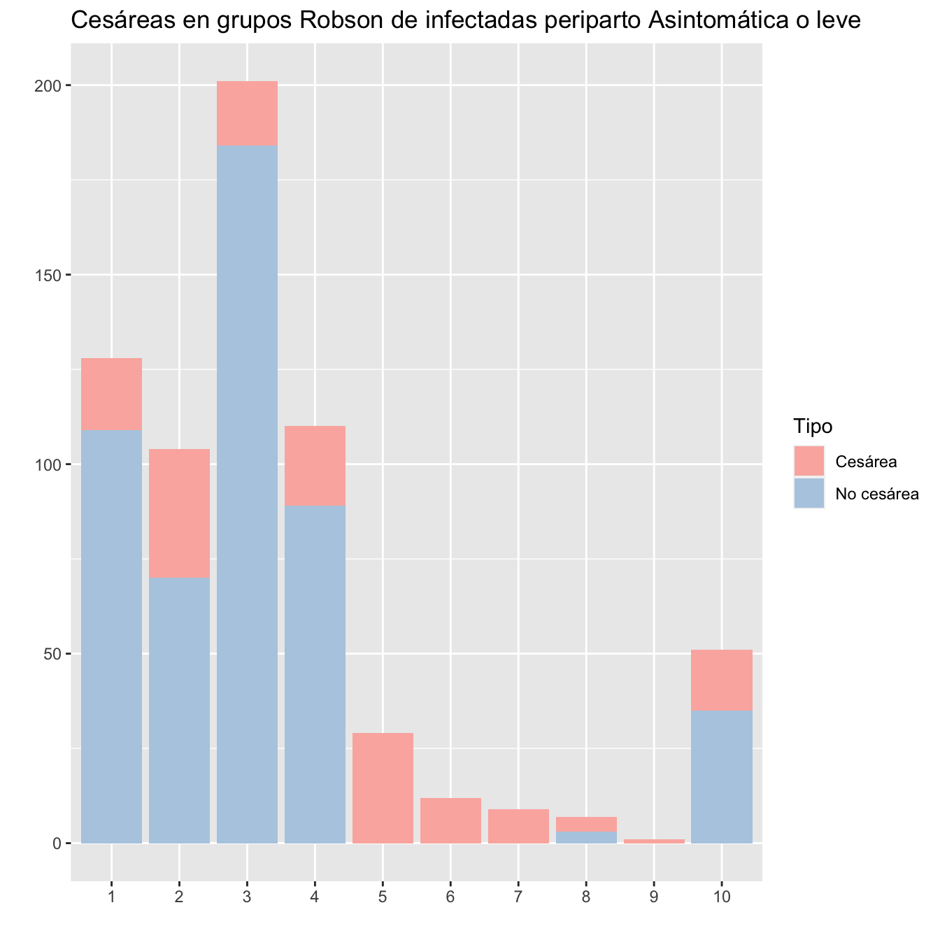
Figura 10.15:
Tipo=factor(rep(c("Cesárea","No cesárea"), each=10))
Grupo=factor(rep(1:10 , 2))
valor=as.vector(TRCaPG[c(2:11),2:1])
data=data.frame(Grupo,Tipo,valor)

ggplot(data, aes(fill=Tipo, y=valor, x=Grupo)) +
  geom_bar(position="stack", stat="identity")+
  ylab("")+
  xlab("")+
  ggtitle("Cesáreas en grupos Robson de infectadas periparto graves")+
scale_fill_brewer(palette = "Pastel1") 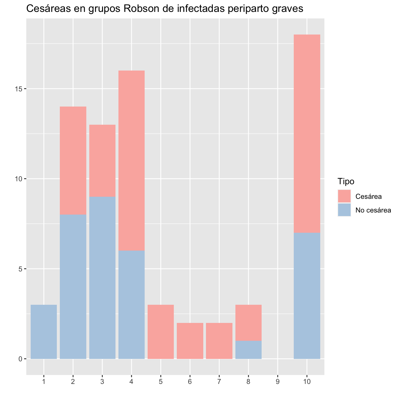
Figura 10.16:
10.6.1 Diferencias?
Qué grupos tienen proporciones de cesáreas significativamente diferentes en las infectadas anteparto y periparto? Algunos!
EE1=t(TRcaPreP)[2:1,2:11]
EE2=t(TRcaPeriP)[2:1,2:11]
OR=rep(0,10)
pp=rep(0,10)
for (i in 1:10){
FT=fisher.test(cbind(EE1[,i],EE2[,i]))
OR[i]=FT$estimate
pp[i]=FT$p.value       }

dt=data.frame(1:10,colSums(EE1),EE1[1,],round(100*prop.table(EE1,margin=2)[1,],2),colSums(EE2),EE2[1,],round(100*prop.table(EE2,margin=2)[1,],2),round(OR,2),round(pp,3))
names(dt)=c("Grupo Robson", "Inf. anteparto", "Cesáreas", "Porcentaje",  "Inf. periparto", "Cesáreas", "Porcentaje","OR","p-valor test de Fisher")
dt %>%
  kbl() %>%
  kable_styling()%>%
scroll_box(width="100%", box_css="border: 0px;")| Grupo Robson | Inf. anteparto | Cesáreas | Porcentaje | Inf. periparto | Cesáreas | Porcentaje | OR | p-valor test de Fisher |
|---|---|---|---|---|---|---|---|---|
| 1 | 127 | 9 | 7.09 | 131 | 19 | 14.50 | 0.45 | 0.071 |
| 2 | 132 | 44 | 33.33 | 118 | 40 | 33.90 | 0.98 | 1.000 |
| 3 | 295 | 9 | 3.05 | 214 | 21 | 9.81 | 0.29 | 0.002 |
| 4 | 206 | 41 | 19.90 | 126 | 31 | 24.60 | 0.76 | 0.338 |
| 5 | 45 | 45 | 100.00 | 32 | 32 | 100.00 | 0.00 | 1.000 |
| 6 | 17 | 17 | 100.00 | 14 | 14 | 100.00 | 0.00 | 1.000 |
| 7 | 15 | 15 | 100.00 | 11 | 11 | 100.00 | 0.00 | 1.000 |
| 8 | 21 | 13 | 61.90 | 10 | 6 | 60.00 | 1.08 | 1.000 |
| 9 | 1 | 1 | 100.00 | 1 | 1 | 100.00 | 0.00 | 1.000 |
| 10 | 70 | 40 | 57.14 | 69 | 27 | 39.13 | 2.06 | 0.042 |
Qué grupos tienen proporciones de cesáreas en infectadas periparto no graves o no infectadas significativamente diferentes? Ninguno:
| Grupo Robson | Casos Peripartos asintomáticos o leve | Cesáreas | Porcentaje | Controles | Cesáreas | Porcentaje | OR | p-valor test de Fisher |
|---|---|---|---|---|---|---|---|---|
| 1 | 128 | 19 | 14.84 | 357 | 43 | 12.04 | 1.27 | 0.441 |
| 2 | 104 | 34 | 32.69 | 220 | 70 | 31.82 | 1.04 | 0.899 |
| 3 | 201 | 17 | 8.46 | 551 | 32 | 5.81 | 1.50 | 0.241 |
| 4 | 110 | 21 | 19.09 | 263 | 43 | 16.35 | 1.21 | 0.548 |
| 5 | 29 | 29 | 100.00 | 56 | 56 | 100.00 | 0.00 | 1.000 |
| 6 | 12 | 12 | 100.00 | 17 | 16 | 94.12 | Inf | 1.000 |
| 7 | 9 | 9 | 100.00 | 20 | 20 | 100.00 | 0.00 | 1.000 |
| 8 | 7 | 4 | 57.14 | 34 | 17 | 50.00 | 1.32 | 1.000 |
| 9 | 1 | 1 | 100.00 | 1 | 1 | 100.00 | 0.00 | 1.000 |
| 10 | 51 | 16 | 31.37 | 76 | 26 | 34.21 | 0.88 | 0.848 |
Qué grupos tienen proporciones de cesáreas en infectadas periparto graves o no infectadas significativamente diferentes? Algunos!
| Grupo Robson | Casos Peripartos Graves | Cesáreas | Porcentaje | Controles | Cesáreas | Porcentaje | OR | p-valor test de Fisher |
|---|---|---|---|---|---|---|---|---|
| 1 | 3 | 0 | 0.00 | 357 | 43 | 12.04 | 0.00 | 1.000 |
| 2 | 14 | 6 | 42.86 | 220 | 70 | 31.82 | 1.60 | 0.391 |
| 3 | 13 | 4 | 30.77 | 551 | 32 | 5.81 | 7.15 | 0.007 |
| 4 | 16 | 10 | 62.50 | 263 | 43 | 16.35 | 8.43 | 0.000 |
| 5 | 3 | 3 | 100.00 | 56 | 56 | 100.00 | 0.00 | 1.000 |
| 6 | 2 | 2 | 100.00 | 17 | 16 | 94.12 | Inf | 1.000 |
| 7 | 2 | 2 | 100.00 | 20 | 20 | 100.00 | 0.00 | 1.000 |
| 8 | 3 | 2 | 66.67 | 34 | 17 | 50.00 | 1.96 | 1.000 |
| 9 | 0 | 0 | 1 | 1 | 100.00 | 0.00 | 1.000 | |
| 10 | 18 | 11 | 61.11 | 76 | 26 | 34.21 | 2.98 | 0.058 |
Qué grupos tienen proporciones de cesáreas en infectadas periparto no graves o graves significativamente diferentes? Bastantes!
EE1=t(TRCaPG)[2:1,2:11]
EE2=t(TRCaPL)[2:1,2:11]
OR=rep(0,10)
pp=rep(0,10)
for (i in 1:10){
FT=fisher.test(cbind(EE1[,i],EE2[,i]))
OR[i]=FT$estimate
pp[i]=FT$p.value       }

dt=data.frame(1:10,colSums(EE1),EE1[1,],round(100*prop.table(EE1,margin=2)[1,],2),colSums(EE2),EE2[1,],round(100*prop.table(EE2,margin=2)[1,],2),round(OR,2),round(pp,3))
names(dt)=c("Grupo Robson", "Periparto Grave", "Cesáreas", "Porcentaje",  "Periparto no Grave", "Cesáreas", "Porcentaje","OR","p-valor test de Fisher")
dt %>%
  kbl() %>%
  kable_styling()%>%
scroll_box(width="100%", box_css="border: 0px;")| Grupo Robson | Periparto Grave | Cesáreas | Porcentaje | Periparto no Grave | Cesáreas | Porcentaje | OR | p-valor test de Fisher |
|---|---|---|---|---|---|---|---|---|
| 1 | 3 | 0 | 0.00 | 128 | 19 | 14.84 | 0.00 | 1.000 |
| 2 | 14 | 6 | 42.86 | 104 | 34 | 32.69 | 1.54 | 0.550 |
| 3 | 13 | 4 | 30.77 | 201 | 17 | 8.46 | 4.75 | 0.028 |
| 4 | 16 | 10 | 62.50 | 110 | 21 | 19.09 | 6.92 | 0.001 |
| 5 | 3 | 3 | 100.00 | 29 | 29 | 100.00 | 0.00 | 1.000 |
| 6 | 2 | 2 | 100.00 | 12 | 12 | 100.00 | 0.00 | 1.000 |
| 7 | 2 | 2 | 100.00 | 9 | 9 | 100.00 | 0.00 | 1.000 |
| 8 | 3 | 2 | 66.67 | 7 | 4 | 57.14 | 1.44 | 1.000 |
| 9 | 0 | 0 | 1 | 1 | 100.00 | 0.00 | 1.000 | |
| 10 | 18 | 11 | 61.11 | 51 | 16 | 31.37 | 3.37 | 0.047 |
CasosPrep=droplevels(Casos[Casos$PreP=="Anteparto",])
CasosPeri=droplevels(Casos[Casos$PreP=="Periparto",])TRCa1wS=table(CasosPrep$Robson,CasosPrep$SINTOMAS_DIAGNOSTICO)[c(2:11,1),]
pTRCa1wS=round(100*prop.table(table(CasosPrep$Robson,CasosPrep$SINTOMAS_DIAGNOSTICO),margin=1)[c(2:11,1),],2)
TRCa2wS=table(CasosPeri$Robson,CasosPeri$SINTOMAS_DIAGNOSTICO)[c(2:11,1),]
pTRCa2wS=round(100*prop.table(table(CasosPeri$Robson,CasosPeri$SINTOMAS_DIAGNOSTICO),margin=1)[c(2:11,1),],2)
DFTRCaWS=data.frame(
Robson=c(1:10,"Pérdidas"),
Tot1w=as.vector(table(CasosPrep$Robson)[c(2:11,1)]),
Asint1w=TRCa1wS[,1],
pAsint1w=pTRCa1wS[,1],
SL1w=TRCa1wS[,2],
pSL1w=pTRCa1wS[,2],
Neum1w=TRCa1wS[,3],
pTRCa1wS[,3],
Tot2w=as.vector(table(CasosPeri$Robson)[c(2:11,1)]),
Asint2w=TRCa2wS[,1],
pAsint2w=pTRCa2wS[,1],
SL2w=TRCa2wS[,2],
pSL2w=pTRCa2wS[,2],
Neum2w=TRCa2wS[,3],
pTRCa2wS[,3])
row.names(DFTRCaWS)=c()
names(DFTRCaWS)=c("Grupo Robson", "Total infectadas anteparto", "Asintomática prepartp", "%", "Leve anteparto", "%", "Grave anteparto", "%","Total infectadas periparto", "Asintomática periparto", "%", "Leve periparto", "%", "Grave peripartoa", "%")
DFTRCaWS %>%
kbl() %>%
kable_styling()%>%
scroll_box(width="100%", box_css="border: 0px;")| Grupo Robson | Total infectadas anteparto | Asintomática prepartp | % | Leve anteparto | % | Grave anteparto | % | Total infectadas periparto | Asintomática periparto | % | Leve periparto | % | Grave peripartoa | % |
|---|---|---|---|---|---|---|---|---|---|---|---|---|---|---|
| 1 | 127 | 24 | 18.90 | 85 | 66.93 | 18 | 14.17 | 131 | 101 | 77.10 | 27 | 20.61 | 3 | 2.29 |
| 2 | 132 | 42 | 31.82 | 65 | 49.24 | 25 | 18.94 | 118 | 78 | 66.10 | 26 | 22.03 | 14 | 11.86 |
| 3 | 295 | 73 | 24.75 | 159 | 53.90 | 63 | 21.36 | 214 | 179 | 83.64 | 22 | 10.28 | 13 | 6.07 |
| 4 | 206 | 44 | 21.36 | 113 | 54.85 | 49 | 23.79 | 126 | 88 | 69.84 | 22 | 17.46 | 16 | 12.70 |
| 5 | 45 | 9 | 20.00 | 23 | 51.11 | 13 | 28.89 | 32 | 21 | 65.62 | 8 | 25.00 | 3 | 9.38 |
| 6 | 17 | 5 | 29.41 | 10 | 58.82 | 2 | 11.76 | 14 | 8 | 57.14 | 4 | 28.57 | 2 | 14.29 |
| 7 | 15 | 3 | 20.00 | 9 | 60.00 | 3 | 20.00 | 11 | 6 | 54.55 | 3 | 27.27 | 2 | 18.18 |
| 8 | 21 | 3 | 14.29 | 15 | 71.43 | 3 | 14.29 | 10 | 5 | 50.00 | 2 | 20.00 | 3 | 30.00 |
| 9 | 1 | 0 | 0.00 | 1 | 100.00 | 0 | 0.00 | 1 | 1 | 100.00 | 0 | 0.00 | 0 | 0.00 |
| 10 | 70 | 18 | 25.71 | 24 | 34.29 | 28 | 40.00 | 69 | 28 | 40.58 | 23 | 33.33 | 18 | 26.09 |
| Pérdidas | 4 | 2 | 50.00 | 1 | 25.00 | 1 | 25.00 | 9 | 7 | 77.78 | 1 | 11.11 | 1 | 11.11 |
Tipo=factor(rep(c("Asintomática","Leve", "Grave"), each=10))
Grupo=factor(rep(1:10 , 3))
valor=as.vector(TRCa1wS[1:10,])
data=data.frame(Grupo,Tipo,valor)

ggplot(data, aes(fill=Tipo, y=valor, x=Grupo)) +
  geom_bar(position="stack", stat="identity")+
  ylab("")+
  xlab("")+
  ggtitle("Grupos sintomáticos en grupos Robson en las infectadas anteparto")+
scale_fill_brewer(palette = "Dark2") 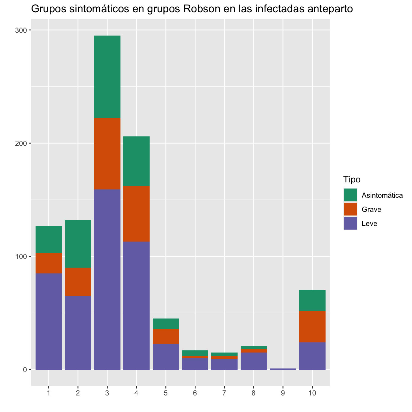
Figura 10.17:
Tipo=ordered(rep(c("Asintomática","Leve", "Grave"), each=10),levels=c("Asintomática","Leve", "Grave"))
Grupo=factor(rep(1:10 , 3))
valor=as.vector(TRCa2wS[1:10,])
data=data.frame(Grupo,Tipo,valor)

ggplot(data, aes(fill=Tipo, y=valor, x=Grupo)) +
  geom_bar(position="stack", stat="identity")+
  ylab("")+
  xlab("")+
  ggtitle("Grupos sintomáticos en grupos Robson en las infectadas periparto")+
scale_fill_brewer(palette = "Dark2") 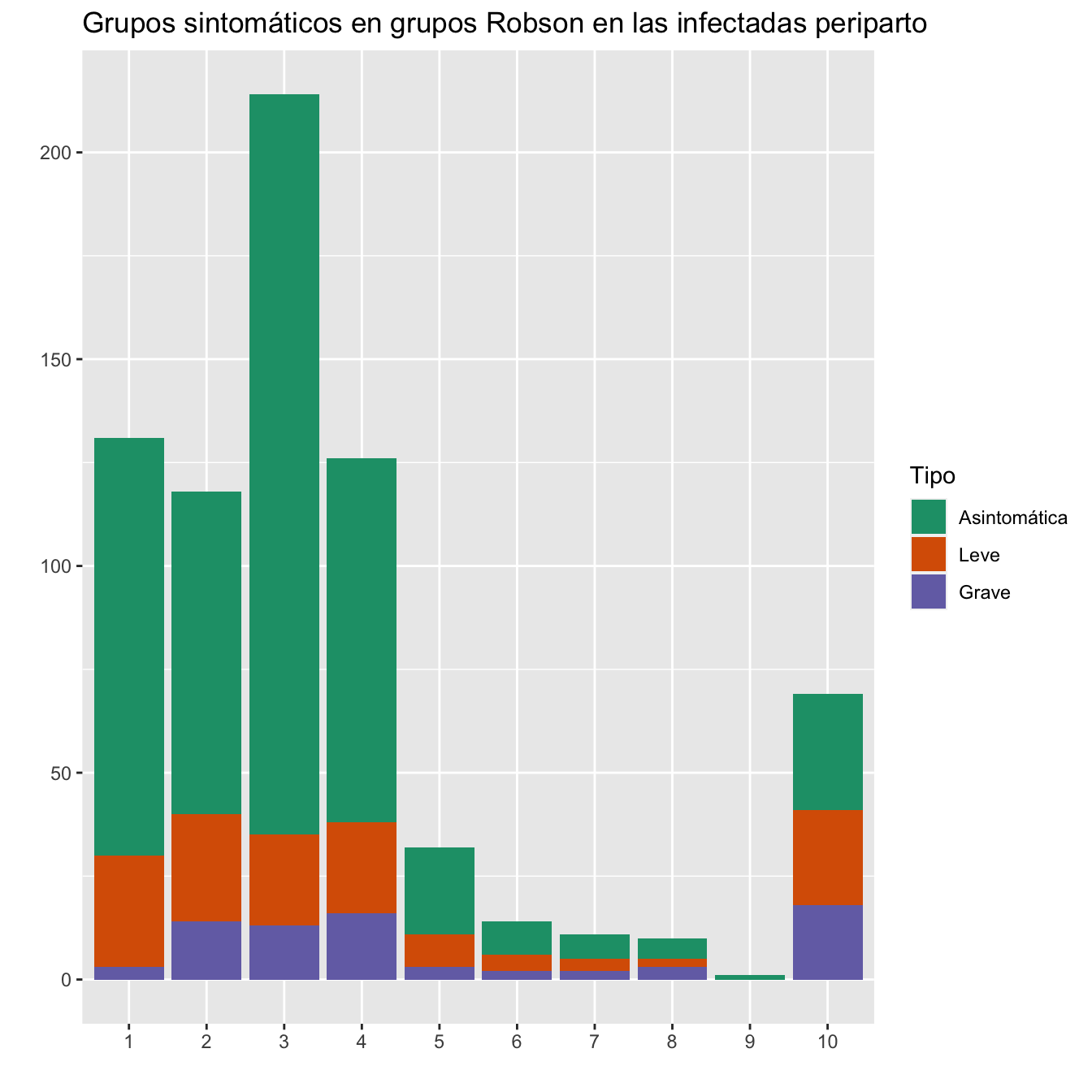
Figura 10.18:
En la tabla que sigue, para cada grupo y cada momento de diagnóatico, el p-valor es del contraste \(\chi^2\) de si la distribución de los síntomas de las infectadas de ese grupo y ese momento es igual o diferente de la distribución de los síntomas de las infectadas de ese grupo en el total de las dos olas.
pp=c()
for (i in c(1:8,10)){
pp[i]=chisq.test(TRCa1wS[i,],p=prop.table(TRCa1wS+TRCa2wS,margin=1)[i,],simulate.p.value=TRUE,B=10000)$p.value
}
for (i in c(11:18,20)){
pp[i]=chisq.test(TRCa2wS[i-10,],p=prop.table(TRCa1wS[i-10,]+TRCa2wS[i-10,]),simulate.p.value=TRUE,B=10000)$p.value
}
tabla=data.frame(
Robson=rep(1:10,2),
Ola=rep(c("Preparto","Periparto"),each=10),
round(pp,4)
)
names(tabla)=c("Grupo Robson","Diagnóstico","p-valor")
row.names(tabla)=c()

tabla %>%
  kbl() %>%
  kable_styling()%>%
scroll_box(width="100%", box_css="border: 0px;")| Grupo Robson | Diagnóstico | p-valor |
|---|---|---|
| 1 | Preparto | 0.0001 |
| 2 | Preparto | 0.0016 |
| 3 | Preparto | 0.0001 |
| 4 | Preparto | 0.0001 |
| 5 | Preparto | 0.0295 |
| 6 | Preparto | 0.5188 |
| 7 | Preparto | 0.4644 |
| 8 | Preparto | 0.3403 |
| 9 | Preparto | |
| 10 | Preparto | 0.3518 |
| 1 | Periparto | 0.0001 |
| 2 | Periparto | 0.0008 |
| 3 | Periparto | 0.0001 |
| 4 | Periparto | 0.0001 |
| 5 | Periparto | 0.0095 |
| 6 | Periparto | 0.4534 |
| 7 | Periparto | 0.3419 |
| 8 | Periparto | 0.0879 |
| 9 | Periparto | |
| 10 | Periparto | 0.3451 |
10.6.2 Enter cesáreas
Dejo de tener en cuenta los grupos 5,6,7,9, donde las cesáreas fueron constantes.
TRCa1wSC=table(CasosPrep$Cesárea,CasosPrep$SINTOMAS_DIAGNOSTICO,CasosPrep$Robson)[2:1,,c(2:11,1)]
pTRCa1wSC=round(100*prop.table(TRCa1wSC,margin=c(2,3)),2)
TRCa2wSC=table(CasosPeri$Cesárea,CasosPeri$SINTOMAS_DIAGNOSTICO,CasosPeri$Robson)[2:1,,c(2:11,1)]
pTRCa2wSC=round(100*prop.table(TRCa2wSC,margin=c(2,3)),2)

DFTRCaWSC=data.frame(
Robson=c(1:10,"Pérdidas"),
Asint1w=TRCa1wS[,1],
pAsint1w=pTRCa1wSC[1,1,],
SL1w=TRCa1wS[,2],
pSL1w=pTRCa1wSC[1,2,],
Neum1w=TRCa1wS[,3],
pNeum1w=pTRCa1wSC[1,3,],
Asint2w=TRCa2wS[,1],
pAsint2w=pTRCa2wSC[1,1,],
SL2w=TRCa2wS[,2],
pSL2w=pTRCa2wSC[1,2,],
Neum2w=TRCa2wS[,3],
pNeum2w=pTRCa2wSC[1,3,]
)
DFTRCaWSC=DFTRCaWSC[c(1:4,8,10),]
row.names(DFTRCaWSC)=c()

names(DFTRCaWSC)=c("Grupo Robson", "Asintomática anteparto", "% cesáreas en Asintomática anteparto", "Leve anteparto", "% cesáreas en Leve anteparto", "Graves anteparto", "% cesáreas en Grave anteparto",  "Asintomática periparto","% cesáreas en Asintomática periparto", "Leve periparto", "% cesáreas en Leve periparto", "Graves periparto", "% cesáreas en Grave periparto")

DFTRCaWSC %>%
  kbl() %>%
  kable_styling()%>%
scroll_box(width="100%", box_css="border: 0px;")| Grupo Robson | Asintomática anteparto | % cesáreas en Asintomática anteparto | Leve anteparto | % cesáreas en Leve anteparto | Graves anteparto | % cesáreas en Grave anteparto | Asintomática periparto | % cesáreas en Asintomática periparto | Leve periparto | % cesáreas en Leve periparto | Graves periparto | % cesáreas en Grave periparto |
|---|---|---|---|---|---|---|---|---|---|---|---|---|
| 1 | 24 | 8.33 | 85 | 4.71 | 18 | 16.67 | 101 | 14.85 | 27 | 14.81 | 3 | 0.00 |
| 2 | 42 | 38.10 | 65 | 29.23 | 25 | 36.00 | 78 | 34.62 | 26 | 26.92 | 14 | 42.86 |
| 3 | 73 | 2.74 | 159 | 3.14 | 63 | 3.17 | 179 | 6.70 | 22 | 22.73 | 13 | 30.77 |
| 4 | 44 | 18.18 | 113 | 21.24 | 49 | 18.37 | 88 | 18.18 | 22 | 22.73 | 16 | 62.50 |
| 8 | 3 | 66.67 | 15 | 53.33 | 3 | 100.00 | 5 | 60.00 | 2 | 50.00 | 3 | 66.67 |
| 10 | 18 | 55.56 | 24 | 41.67 | 28 | 71.43 | 28 | 21.43 | 23 | 43.48 | 18 | 61.11 |
En la tabla que sigue, para cada grupo y cada momento, el p-valor es del contraste de si la distribución de cesáreas en los grupos sintomáticos de las infectadas de ese grupo y ese momento es igual o diferente de la distribución de cesáreas en los grupos sintomáticos de las infectadas.
pp=c()
for(i in c(1:4,8,10)){
EEw=TRCa1wSC[,,i]
EE=TRCa1wSC[,,i]+TRCa2wSC[,,i]
pp[i]=Prop.trend.test(EEw[1,],colSums(EEw))
}
for(i in c(11:14,18,20)){
EEw=TRCa2wSC[,,i-10]
EE=TRCa1wSC[,,i-10]+TRCa2wSC[,,i-10]
pp[i]=Prop.trend.test(EEw[1,],colSums(EEw))
}
pp=pp[!is.na(pp)]

tabla=data.frame(
Robson=rep(c(1:4,8,10),2),
Ola=rep(c("Preparto","Periparto"),each=6),
round(pp,4)
)
names(tabla)=c("Grupo Robson","Diagnóstico","p-valor")
row.names(tabla)=c()

tabla %>%
  kbl() %>%
  kable_styling()%>%
scroll_box(width="100%", box_css="border: 0px;")| Grupo Robson | Diagnóstico | p-valor |
|---|---|---|
| 1 | Preparto | 0.2598 |
| 2 | Preparto | 0.7788 |
| 3 | Preparto | 0.9851 |
| 4 | Preparto | 0.9103 |
| 8 | Preparto | 0.7889 |
| 10 | Preparto | 0.5224 |
| 1 | Periparto | 0.8009 |
| 2 | Periparto | 0.7654 |
| 3 | Periparto | 0.0103 |
| 4 | Periparto | 0.0299 |
| 8 | Periparto | 0.9824 |
| 10 | Periparto | 0.1917 |
En la tabla que sigue, para cada grupo Robson y para cada sintomático:
- OR: la OR de cesárea relativa a ser anteparto
- p-valor: el p-valor del test de Fisher bilateral para comparar las proporciones de cesáreas en ese grupo Robson y ese grupo sintomático entre los dos momentos de diagnóstico
ppA=c()
ppSL=c()
ppN=c()
ORA=c()
ORSL=c()
ORN=c()
for(i in c(1:4,8,10)){
EE1w=TRCa1wSC[,,i]
EE2w=TRCa2wSC[,,i]
ORA[i]=fisher.test(cbind(EE1w[,1],EE2w[,1]))$estimate
ORSL[i]=fisher.test(cbind(EE1w[,2],EE2w[,2]))$estimate
ORN[i]=fisher.test(cbind(EE1w[,3],EE2w[,3]))$estimate

ppA[i]=fisher.test(cbind(EE1w[,1],EE2w[,1]))$p.value
ppSL[i]=fisher.test(cbind(EE1w[,2],EE2w[,2]))$p.value
ppN[i]=fisher.test(cbind(EE1w[,3],EE2w[,3]))$p.value
}
ppA=ppA[!is.na(ppA)]
ppSL=ppSL[!is.na(ppSL)]
ppN=ppN[!is.na(ppN)]

ORA=ORA[!is.na(ORA)]
ORSL=ORSL[!is.na(ORSL)]
ORN=ORN[!is.na(ORN)]


tabla=data.frame(
Robson=c(1:4,8,10),
round(ORA,4),
round(ppA,4),
round(ORSL,4),
round(ppSL,4),
round(ORN,4),
round(ppN,4)
)
names(tabla)=c("Grupo Robson", "OR Asintomática", "p-valor Asintomática","OR Leve","p-valor Leve","OR Grave","p-valor Grave")
row.names(tabla)=c()

tabla %>%
  kbl() %>%
  kable_styling()%>%
scroll_box(width="100%", box_css="border: 0px;")| Grupo Robson | OR Asintomática | p-valor Asintomática | OR Leve | p-valor Leve | OR Grave | p-valor Grave |
|---|---|---|---|---|---|---|
| 1 | 0.5235 | 0.5231 | 0.2880 | 0.0939 | Inf | 1.0000 |
| 2 | 1.1609 | 0.8420 | 1.1197 | 1.0000 | 0.7556 | 0.7397 |
| 3 | 0.3932 | 0.3623 | 0.1129 | 0.0028 | 0.0782 | 0.0068 |
| 4 | 1.0000 | 1.0000 | 0.9175 | 1.0000 | 0.1405 | 0.0015 |
| 8 | 1.2866 | 1.0000 | 1.1339 | 1.0000 | Inf | 1.0000 |
| 10 | 4.4157 | 0.0271 | 0.9300 | 1.0000 | 1.5745 | 0.5297 |
TCaAsin=table(Casos$Robson[Casos$SINTOMAS_CAT==1],Casos$Cesárea[Casos$SINTOMAS_CAT==1])[2:11,2:1]
TCaSL=table(Casos$Robson[Casos$SINTOMAS_CAT==2],Casos$Cesárea[Casos$SINTOMAS_CAT==2])[2:11,2:1]
TCaNeu=table(Casos$Robson[Casos$SINTOMAS_CAT==3],Casos$Cesárea[Casos$SINTOMAS_CAT==3])[2:11,2:1]
dades=data.frame(1:10,
rowSums(TCaAsin),TCaAsin[,1],round(100*prop.table(TCaAsin,margin=1)[,1],2),
rowSums(TCaSL),TCaSL[,1],round(100*prop.table(TCaSL,margin=1)[,1],2),
rowSums(TCaNeu),TCaNeu[,1],round(100*prop.table(TCaNeu,margin=1)[,1],2))
      names(dades)=c("Grupo Robson", "Inf. Asintomática", "Cesáreas", "Porcentaje",
                     "Inf. Leve", "Cesáreas", "Porcentaje",
                     "Inf. Grave", "Cesáreas", "Porcentaje")
dades %>%
  kbl() %>%
  kable_styling()%>%
scroll_box(width="100%", box_css="border: 0px;")| Grupo Robson | Inf. Asintomática | Cesáreas | Porcentaje | Inf. Leve | Cesáreas | Porcentaje | Inf. Grave | Cesáreas | Porcentaje |
|---|---|---|---|---|---|---|---|---|---|
| 1 | 125 | 17 | 13.60 | 112 | 8 | 7.14 | 21 | 3 | 14.29 |
| 2 | 120 | 43 | 35.83 | 91 | 26 | 28.57 | 39 | 15 | 38.46 |
| 3 | 252 | 14 | 5.56 | 181 | 10 | 5.52 | 76 | 6 | 7.89 |
| 4 | 132 | 24 | 18.18 | 135 | 29 | 21.48 | 65 | 19 | 29.23 |
| 5 | 30 | 30 | 100.00 | 31 | 31 | 100.00 | 16 | 16 | 100.00 |
| 6 | 13 | 13 | 100.00 | 14 | 14 | 100.00 | 4 | 4 | 100.00 |
| 7 | 9 | 9 | 100.00 | 12 | 12 | 100.00 | 5 | 5 | 100.00 |
| 8 | 8 | 5 | 62.50 | 17 | 9 | 52.94 | 6 | 5 | 83.33 |
| 9 | 1 | 1 | 100.00 | 1 | 1 | 100.00 | 0 | 0 | |
| 10 | 46 | 16 | 34.78 | 47 | 20 | 42.55 | 46 | 31 | 67.39 |
En la lista que sigue, los p-valores son los del contraste si las proporciones de cesáreas en los grupos 1,2,3,4,8 y 10 son las mismas o no en los dos grupos sintomáticos comparados:
pp=c()
EE=dades[c(1:4,8,10),c(2,3,5,6,8,9)]
pp[1]=Prop.trend.test(EE[,2],EE[,1])
pp[2]=Prop.trend.test(EE[,2],EE[,1])
pp[3]=Prop.trend.test(EE[,4],EE[,3])- Asintomática contra Leve: \(2\times 10^{-9}\)
- Asintomática contra Grave: \(2\times 10^{-9}\)
- Leve contra Grave: \(8\times 10^{-9}\)
10.7 Bonus Track
Datos sobre un hospital valenciano de 2010 a 2018 (https://doi.org/10.3390/ijerph17051575)
DatosAnteriores=data.frame(matrix(c(638,    5529    ,921,   2527    ,338,   5283    ,402,   1578    ,23,    118 ,304,   320 ,136,   158 ,133,   229 ,35,    35  ,222,   729),nrow=10,byrow=T))
names(DatosAnteriores)=c("Cesáreas","Gestantes")
DatosAnteriores$Robson=1:10
DatosAnteriores=DatosAnteriores[,c(3,2,1)]
DatosAnteriores$Porcentaje=round(100*DatosAnteriores$Cesáreas/DatosAnteriores$Gestantes,2)

DatosAnteriores %>%
  kbl() %>%
  kable_styling()%>%
scroll_box(width="100%", box_css="border: 0px;")| Robson | Gestantes | Cesáreas | Porcentaje |
|---|---|---|---|
| 1 | 5529 | 638 | 11.54 |
| 2 | 2527 | 921 | 36.45 |
| 3 | 5283 | 338 | 6.40 |
| 4 | 1578 | 402 | 25.48 |
| 5 | 118 | 23 | 19.49 |
| 6 | 320 | 304 | 95.00 |
| 7 | 158 | 136 | 86.08 |
| 8 | 229 | 133 | 58.08 |
| 9 | 35 | 35 | 100.00 |
| 10 | 729 | 222 | 30.45 |
Se ajustan vuestros grupos Robson a esa distribución?
Ant=as.vector(prop.table(DatosAnteriores$Gestantes))
Aqui=as.vector(prop.table(table(c(Casos$Robson,Controls$Robson))[2:11]))
AquiC=as.vector(prop.table(table(c(Controls$Robson))[2:11]))
Distrs=data.frame(Robson=1:10,round(100*Ant,2),round(100*Aqui,2),round(100*AquiC,2))
names(Distrs)=c("Robson","Anterior (%)", "Vuestra global (%)", "Vuestra controles (%)")
Distrs %>%
  kbl() %>%
  kable_styling()%>%
scroll_box(width="100%", box_css="border: 0px;")| Robson | Anterior (%) | Vuestra global (%) | Vuestra controles (%) |
|---|---|---|---|
| 1 | 33.50 | 18.92 | 22.38 |
| 2 | 15.31 | 14.46 | 13.79 |
| 3 | 32.01 | 32.62 | 34.55 |
| 4 | 9.56 | 18.31 | 16.49 |
| 5 | 0.71 | 4.09 | 3.51 |
| 6 | 1.94 | 1.48 | 1.07 |
| 7 | 0.96 | 1.42 | 1.25 |
| 8 | 1.39 | 2.00 | 2.13 |
| 9 | 0.21 | 0.09 | 0.06 |
| 10 | 4.42 | 6.62 | 4.76 |
Global: No
##
##  Chi-squared test for given probabilities
##
## data:  table(c(Casos$Robson, Controls$Robson))[2:11]
## X-squared = 1044, df = 9, p-value < 2.2e-16
Vuestros controles: No
chisq.test(table(Controls$Robson)[2:11],p=prop.table(DatosAnteriores$Gestantes),simulate.p.value = TRUE, B=5000)##
## Chi-squared test for given probabilities with simulated p-value (based
## on 5000 replicates)
##
## data: table(Controls$Robson)[2:11]
## X-squared = 335.18, df = NA, p-value = 2e-04En qué grupos los porcentajes de cesáreas en vuestra muestra fueron diferentes del histórico? En la tabla que sigue
OR Odds ratio de cesárea en (ese grupo) en la muestra actual respecto del histórico
p-valor: p-valor del test de Fisher comparando ese grupo en el actual y el histórico
TTG=table(c(Casos$Cesárea,Controls$Cesárea),c(Casos$Robson,Controls$Robson))[2:1,2:11]
TTCa=table(c(Casos$Cesárea),c(Casos$Robson))[2:1,2:11]
TTGC=table(c(Controls$Cesárea),c(Controls$Robson))[2:1,2:11]
TTAnt=rbind(DatosAnteriores$Cesáreas,DatosAnteriores$Gestantes-DatosAnteriores$Cesáreas)
ppG=rep(0,10)
ppCa=rep(0,10)
ppC=rep(0,10)
ORG=rep(0,10)
ORC=rep(0,10)
ORCa=rep(0,10)

for (i in 1:10){
FTG=fisher.test(cbind(TTG[,i], TTAnt[,i]))
FTCG=fisher.test(cbind(TTGC[,i], TTAnt[,i]))
FTCa=fisher.test(cbind(TTCa[,i], TTAnt[,i]))
ppG[i]=FTG$p.value
ppC[i]=FTCG$p.value
ppCa[i]=FTCG$p.value
ORCa[i]=FTG$estimate

ORG[i]=FTG$estimate
ORC[i]=FTCG$estimate
}

tabla=data.frame(1:10,round(ORG,2),round(ppG,4),round(ORC,2),round(ppC,4),round(ORCa,2),round(ppCa,4))
names(tabla)=c("Robson", "OR global", "p-valor global", "OR controles", "p-valor controles", "OR casos", "p-valor casos")

tabla %>%
  kbl() %>%
  kable_styling()%>%
scroll_box(width="100%", box_css="border: 0px;")| Robson | OR global | p-valor global | OR controles | p-valor controles | OR casos | p-valor casos |
|---|---|---|---|---|---|---|
| 1 | 1.00 | 1.0000 | 1.05 | 0.7334 | 1.00 | 0.7334 |
| 2 | 0.85 | 0.1292 | 0.81 | 0.1877 | 0.85 | 0.1877 |
| 3 | 0.91 | 0.5337 | 0.90 | 0.6465 | 0.91 | 0.6465 |
| 4 | 0.70 | 0.0027 | 0.57 | 0.0011 | 0.70 | 0.0011 |
| 5 | Inf | 0.0000 | Inf | 0.0000 | Inf | 0.0000 |
| 6 | 2.47 | 0.7096 | 0.84 | 0.5943 | 2.47 | 0.5943 |
| 7 | Inf | 0.0051 | Inf | 0.1397 | Inf | 0.1397 |
| 8 | 0.90 | 0.7764 | 0.72 | 0.4583 | 0.90 | 0.4583 |
| 9 | 0.00 | 1.0000 | 0.00 | 1.0000 | 0.00 | 1.0000 |
| 10 | 1.74 | 0.0007 | 1.19 | 0.5151 | 1.74 | 0.5151 |