Lección 1 Descripción de la muestra global
1.1 Antecedentes maternos
Hay 1668 infectadas y 1607 no infectadas.
##
##    0    1
## 1666 2##
## 0
## 1607Entre las infectadas hubo 2 defunciones, las dos en la 1a ola. Esto da una letalidad estimada del 0.12% (IC-95% de Clopper-Pearson [0.015, 0.432]). No hubo ninguna defunción entre los controles.
1.1.1 Edades
data =data.frame(
  name=c(rep("Infectadas",length(I)), rep("No infectadas",length(NI))),
  Edades=c(I,NI)
  )

sample_size = data %>% group_by(name) %>% summarize(num=n())

data %>%
 left_join(sample_size) %>%
  mutate(myaxis = paste0(name, "\n", "n=", num)) %>%
  ggplot( aes(x=myaxis, y=Edades, fill=name)) +
    geom_violin(width=1) +
    geom_boxplot(width=0.1, color="black", alpha=0.2,outlier.fill="black",
               outlier.size=1) +
    theme(
      legend.position="none",
      plot.title = element_text(size=11)
    ) +
    xlab("")+
  ylab("Edades (años)")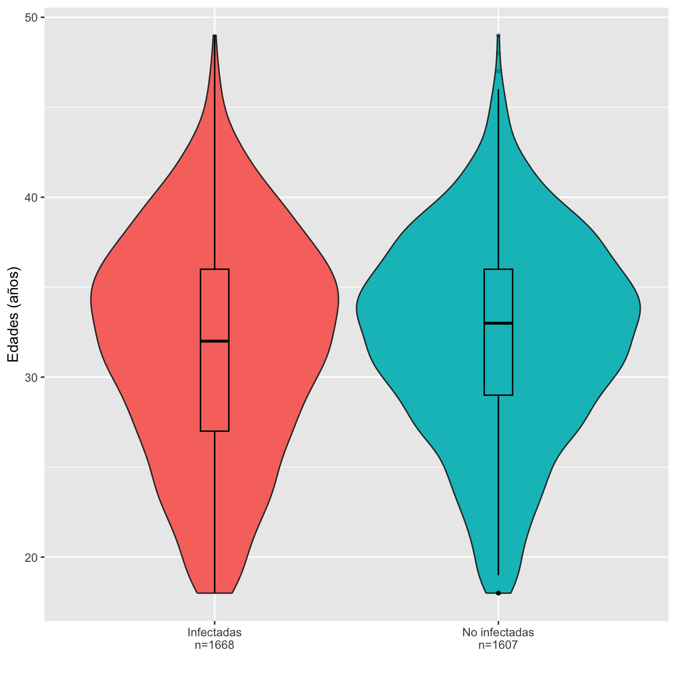
Figura 1.1:
Dades=rbind(c(min(I,na.rm=TRUE),max(I,na.rm=TRUE), round(mean(I,na.rm=TRUE),1),round(median(I,na.rm=TRUE),1),round(quantile(I,c(0.25,0.75),na.rm=TRUE),1), round(sd(I,na.rm=TRUE),1)),
            c(min(NI,na.rm=TRUE),max(NI,na.rm=TRUE), round(mean(NI,na.rm=TRUE),1),round(median(NI,na.rm=TRUE),1),round(quantile(NI,c(0.25,0.75),na.rm=TRUE),1),round(sd(NI,na.rm=TRUE),1)))

colnames(Dades)=c("Edad mínima","Edad máxima","Edad media", "Edad mediana", "1er cuartil", "3er cuartil", "Desv. típica")
rownames(Dades)=c("Infectadas", "No infectadas")

Dades %>%
  kbl() %>%
  kable_styling() %>%
scroll_box(width="100%", box_css="border: 0px;")| Edad mínima | Edad máxima | Edad media | Edad mediana | 1er cuartil | 3er cuartil | Desv. típica | |
|---|---|---|---|---|---|---|---|
| Infectadas | 18 | 49 | 31.9 | 32 | 27 | 36 | 6.2 |
| No infectadas | 18 | 49 | 32.2 | 33 | 29 | 36 | 5.6 |
Ajuste de las edades de infectadas y no infectadas a distribuciones normales: test de Shapiro-Wilks, p-valores \(6\times 10^{-11}\) y \(2\times 10^{-9}\), respectivamente
Igualdad de edades medias: test t, p-valor 0.15, IC del 95% para la diferencia de medias [-0.71, 0.11] años
Igualdad de desviaciones típicas: test de Fligner-Killeen, p-valor \(5\times 10^{-5}\)
En las tablas como la que sigue:
- Los porcentajes se han calculado en la muestra sin pérdidas
- OR: la odds ratio univariante estimada de infectarse relativa a la franja de edad
- IC: el intervalo de confianza del 95% para la OR
- p-valor ajustado: p-valores de tests de Fisher bilaterales ajustados por Bonferroni calculados para la muestra sin pérdidas
I.cut=cut(I,breaks=c(0,30,40,100),labels=c("18-30","31-40",">40"))
NI.cut=cut(NI,breaks=c(0,30,40,100),labels=c("18-30","31-40",">40"))
Tabla.DMGm(I.cut,NI.cut,c("18-30","31-40",">40"))| Infectadas (N) | Infectadas (%) | No infectadas (N) | No infectadas (%) | OR | Extr. Inf. IC | Extr. Sup. IC | p-valor ajustado | |
|---|---|---|---|---|---|---|---|---|
| 18-30 | 647 | 38.9 | 567 | 35.8 | 1.14 | 0.99 | 1.32 | 0.2117 |
| 31-40 | 901 | 54.2 | 931 | 58.7 | 0.83 | 0.72 | 0.96 | 0.0293 |
| >40 | 115 | 6.9 | 87 | 5.5 | 1.28 | 0.95 | 1.73 | 0.3224 |
| Datos perdidos | 5 | 22 |
df =data.frame(
  Factor=c(rep("Infectadas",length(I)), rep("No infectadas",length(NI))),
  Edades=c( I.cut,NI.cut )
)

base=ordered(rep(c("18-30","31-40",">40"), each=2),levels=c("18-30", "31-40",   ">40"))
Grupo=rep(c("Infectada","No infectada") , length(levels(I.cut)))
valor=as.vector(prop.table(table(df), margin=1))
data <- data.frame(base,Grupo,valor)


ggplot(data, aes(fill=base , y=valor, x=Grupo)) +
  geom_bar(position="dodge", stat="identity")+
  ylab("")+
  scale_fill_brewer(palette = "Accent")+
  labs(fill = "Grupo de edad")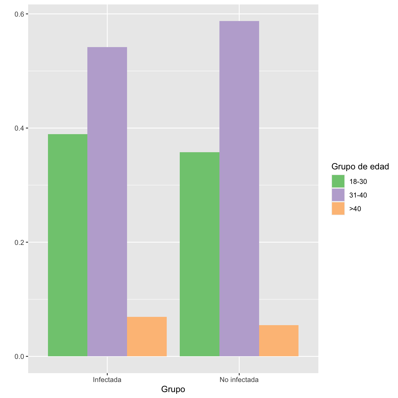
Figura 1.2:
df =data.frame(
  Factor=c(rep("Infectadas",length(I)), rep("No infectadas",length(NI))),
  Edades=c( I.cut,NI.cut )
)

base=ordered(rep(c("18-30","31-40",">40"), each=2),levels=c("18-30", "31-40",   ">40"))
Grupo=rep(c("Infectada","No infectada") , length(levels(I.cut)))
valor=as.vector(prop.table(table(df), margin=2))
data <- data.frame(base,Grupo,valor)


ggplot(data, aes(fill=Grupo, y=valor, x=base)) +
  geom_bar(position="dodge", stat="identity")+
xlab("Grupos de edad")+
  ylab("")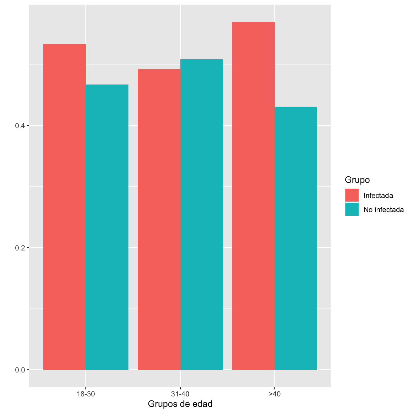
Figura 1.3:
- Igualdad de composiciones por edades de los grupos de casos y de controles: test \(\chi^2\), p-valor 0.0205.
1.1.2 Etnias
I=Casos$Etnia
I[I=="Asia"]="Asiática"
I=factor(I)
NI=factor(Controls$Etnia)
Tabla.DMGm(I,NI,c("Árabe", "Asiática", "Blanca", "Latinoamericana","Negra"),r=6)| Infectadas (N) | Infectadas (%) | No infectadas (N) | No infectadas (%) | OR | Extr. Inf. IC | Extr. Sup. IC | p-valor ajustado | |
|---|---|---|---|---|---|---|---|---|
| Árabe | 141 | 8.5 | 139 | 8.7 | 0.97 | 0.76 | 1.25 | 1.000000 |
| Asiática | 49 | 2.9 | 41 | 2.6 | 1.15 | 0.74 | 1.80 | 1.000000 |
| Blanca | 924 | 55.6 | 1243 | 77.7 | 0.36 | 0.31 | 0.42 | 0.000000 |
| Latinoamericana | 505 | 30.4 | 155 | 9.7 | 4.06 | 3.33 | 4.97 | 0.000000 |
| Negra | 44 | 2.6 | 21 | 1.3 | 2.04 | 1.18 | 3.63 | 0.047009 |
| Datos perdidos | 5 | 8 |
df =data.frame(
  Factor=c(rep("Infectadas",length(I)), rep("No infectadas",length(NI))),
  Etnias=c(I,NI)
)
base=rep(levels(I) , each=2)
Grupo=rep(c("Infectada","No infectada") , length(levels(I)))
valor=as.vector(prop.table(table(df), margin=1))
data <- data.frame(base,Grupo,valor)


ggplot(data, aes(fill=base , y=valor, x=Grupo)) +
  geom_bar(position="dodge", stat="identity")+
  ylab("")+
  scale_fill_brewer(palette = "Accent")+
  labs(fill = "Etnia")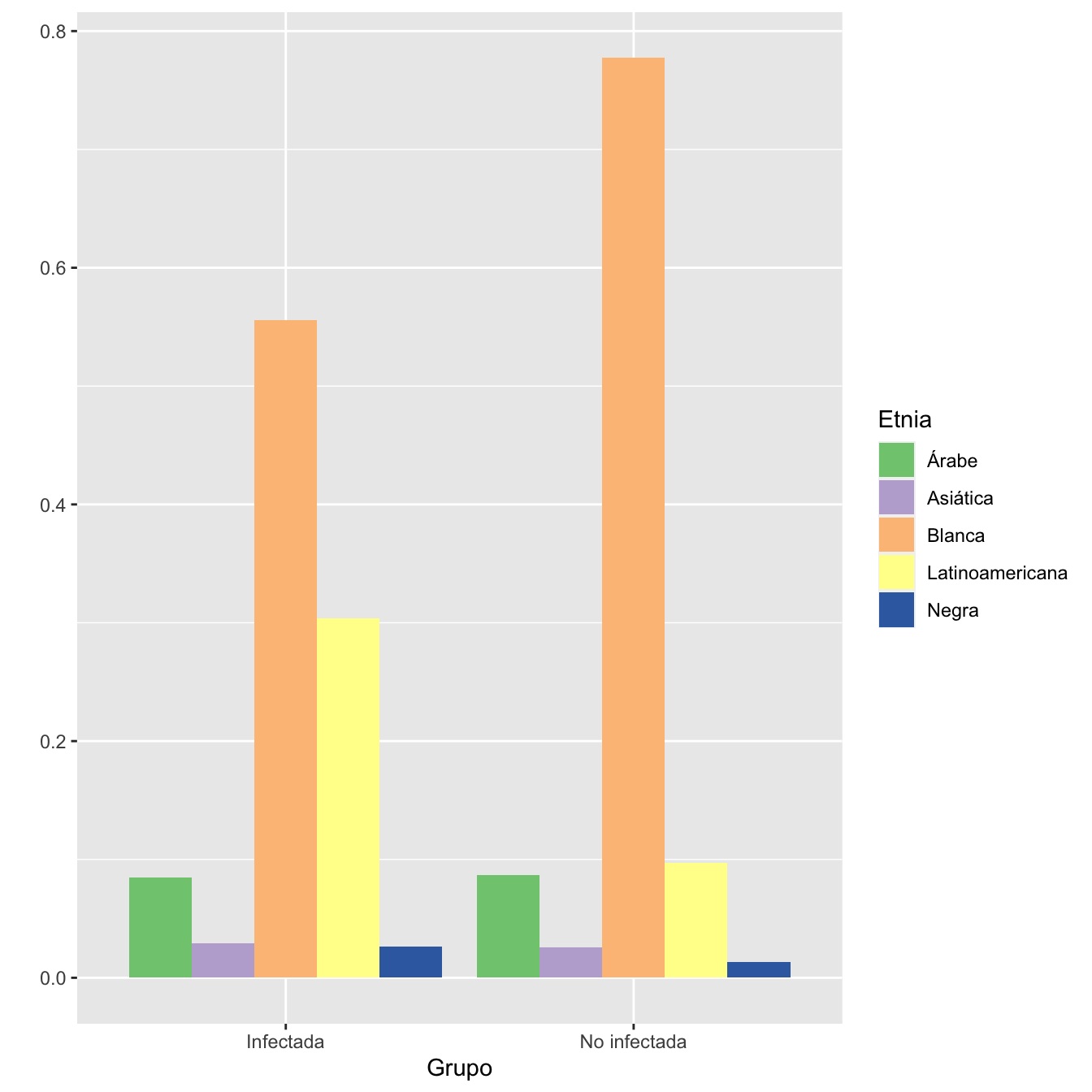
Figura 1.4:
df =data.frame(
  Factor=c(rep("Infectadas",length(I)), rep("No infectadas",length(NI))),
  Etnias=c(I,NI)
)
base=rep(levels(I) , each=2)
Grupo=rep(c("Infectada","No infectada") , length(levels(I)))
valor=as.vector(prop.table(table(df), margin=2))
data <- data.frame(base,Grupo,valor)


ggplot(data, aes(fill=Grupo, y=valor, x=base)) +
  geom_bar(position="dodge", stat="identity")+
xlab("Etnias")+
  ylab("")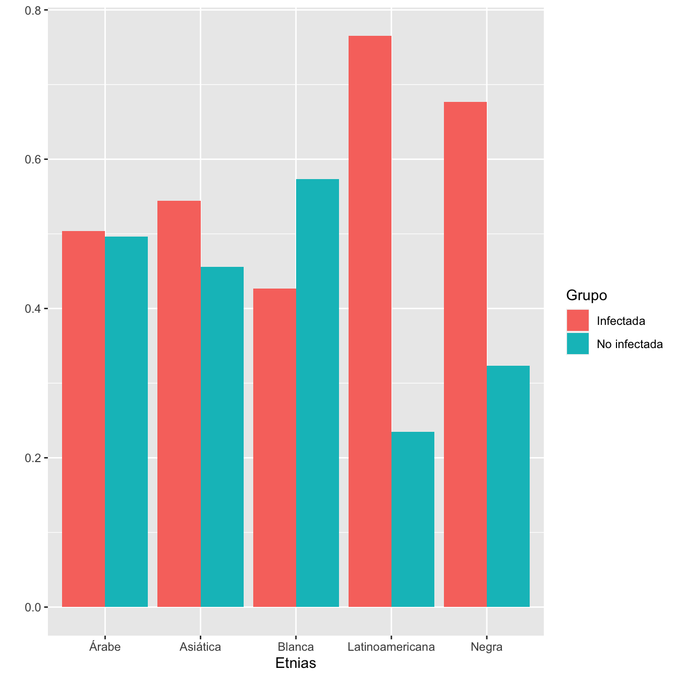
Figura 1.5:
- Composiciones por etnias de los grupos de casos y de controles: test \(\chi^2\), p-valor \(8\times 10^{-51}\)
1.1.3 Hábito tabáquico (juntando fumadoras y ex-fumadoras en una sola categoría)
En las tablas como la que sigue (para antecedentes):
- Los porcentajes se calculan para la muestra sin pérdidas
- La OR es la de infección relativa al antecedente
- El IC es el IC 95% para la OR
- El p-valor es el del test de Fisher bilateral sin tener en cuenta los datos perdidos
| Infectadas (N) | Infectadas (%) | No infectadas (N) | No infectadas (%) | OR | Extr. Inf. IC | Extr. Sup. IC | p-valor | |
|---|---|---|---|---|---|---|---|---|
| Fumadora | 153 | 9.5 | 193 | 12.8 | 0.72 | 0.57 | 0.9 | 0.0036 |
| No fumadora | 1454 | 90.5 | 1312 | 87.2 | ||||
| Datos perdidos | 61 | 102 |
1.1.4 Obesidad
| Infectadas (N) | Infectadas (%) | No infectadas (N) | No infectadas (%) | OR | Extr. Inf. IC | Extr. Sup. IC | p-valor | |
|---|---|---|---|---|---|---|---|---|
| Obesa | 305 | 18.3 | 249 | 16.4 | 1.14 | 0.94 | 1.37 | 0.1748 |
| No obesa | 1363 | 81.7 | 1266 | 83.6 | ||||
| Datos perdidos | 0 | 92 |
1.1.5 Hipertensión pregestacional
I=Casos$Hipertensión.pregestacional
NI=Controls$Hipertensión.pregestacional
Tabla.DMG(I,NI,"No HTA","HTA")| Infectadas (N) | Infectadas (%) | No infectadas (N) | No infectadas (%) | OR | Extr. Inf. IC | Extr. Sup. IC | p-valor | |
|---|---|---|---|---|---|---|---|---|
| HTA | 25 | 1.5 | 17 | 1.1 | 1.34 | 0.69 | 2.66 | 0.4372 |
| No HTA | 1643 | 98.5 | 1497 | 98.9 | ||||
| Datos perdidos | 0 | 93 |
1.1.6 Diabetes Mellitus
| Infectadas (N) | Infectadas (%) | No infectadas (N) | No infectadas (%) | OR | Extr. Inf. IC | Extr. Sup. IC | p-valor | |
|---|---|---|---|---|---|---|---|---|
| DM | 35 | 2.1 | 28 | 1.7 | 1.21 | 0.71 | 2.07 | 0.5251 |
| No DM | 1633 | 97.9 | 1579 | 98.3 | ||||
| Datos perdidos | 0 | 0 |
1.1.7 Enfermedades cardíacas crónicas
| Infectadas (N) | Infectadas (%) | No infectadas (N) | No infectadas (%) | OR | Extr. Inf. IC | Extr. Sup. IC | p-valor | |
|---|---|---|---|---|---|---|---|---|
| ECC | 19 | 1.1 | 27 | 1.8 | 0.65 | 0.34 | 1.21 | 0.1806 |
| No ECC | 1649 | 98.9 | 1515 | 98.2 | ||||
| Datos perdidos | 0 | 65 |
1.1.8 Enfermedades pulmonares crónicas (incluyendo asma)
INA=Casos$Enfermedad.pulmonar.crónica.no.asma
NINA=Controls$Enfermedad.pulmonar.crónica.no.asma
NINA[NINA==0]="No"
NINA[NINA==1]="Sí"
IA=Casos$Diagnóstico.clínico.de.Asma
NIA=Controls$Diagnóstico.clínico.de.Asma
NIA[NIA==0]="No"
NIA[NIA==1]="Sí"

I=rep(NA,n_I)
for (i in 1:n_I){I[i]=max(INA[i],IA[i],na.rm=TRUE)}
NI=rep(NA,n_NI)
for (i in 1:n_NI){NI[i]=max(NINA[i],NIA[i],na.rm=TRUE)}
NI[NI==-Inf]=NA


Tabla.DMG(I,NI,"No EPC","EPC")| Infectadas (N) | Infectadas (%) | No infectadas (N) | No infectadas (%) | OR | Extr. Inf. IC | Extr. Sup. IC | p-valor | |
|---|---|---|---|---|---|---|---|---|
| EPC | 74 | 4.4 | 54 | 3.5 | 1.28 | 0.88 | 1.86 | 0.2061 |
| No EPC | 1594 | 95.6 | 1487 | 96.5 | ||||
| Datos perdidos | 0 | 66 |
1.1.9 Paridad
| Infectadas (N) | Infectadas (%) | No infectadas (N) | No infectadas (%) | OR | Extr. Inf. IC | Extr. Sup. IC | p-valor | |
|---|---|---|---|---|---|---|---|---|
| Nulípara | 606 | 36.7 | 644 | 40.4 | 0.86 | 0.74 | 0.99 | 0.0333 |
| Multípara | 1046 | 63.3 | 952 | 59.6 | ||||
| Datos perdidos | 16 | 11 |
1.1.10 Gestación múltiple
I=Casos$Gestación.Múltiple
NI=Controls$Gestación.Múltiple
Tabla.DMG(I,NI,"Gestación única","Gestación múltiple")| Infectadas (N) | Infectadas (%) | No infectadas (N) | No infectadas (%) | OR | Extr. Inf. IC | Extr. Sup. IC | p-valor | |
|---|---|---|---|---|---|---|---|---|
| Gestación múltiple | 31 | 1.9 | 34 | 2.1 | 0.88 | 0.52 | 1.48 | 0.6182 |
| Gestación única | 1637 | 98.1 | 1573 | 97.9 | ||||
| Datos perdidos | 0 | 0 |
1.2 Desenlaces
1.2.1 Anomalías congénitas
En las tablas como la que sigue (para desenlaces):
- Los porcentajes se calculan para la muestra sin pérdidas
- RA y RR: riesgo absoluto y relativo del desenlace relativo a la infección
- Los IC son el IC 95% para RA y RR
- El p-valor es el del test de Fisher bilateral sin tener en cuenta los datos perdidos
I=Casos$Diagnóstico.de.malformación.ecográfica._.semana.20._
NI=Controls$Diagnóstico.de.malformación.ecográfica._.semana.20._
Tabla.DMGC(I,NI,"No anomalía congénita","Anomalía congénita")| Infectadas (N) | Infectadas (%) | No infectadas (N) | No infectadas (%) | RA | Extr. Inf. IC RA | Extr. Sup. IC RA | RR | Extr. Inf. IC RA | Extr. Sup. IC RR | p-valor | |
|---|---|---|---|---|---|---|---|---|---|---|---|
| Anomalía congénita | 28 | 1.7 | 16 | 1 | 0.0072 | -0.0015 | 0.0159 | 1.71 | 0.94 | 3.13 | 0.0946 |
| No anomalía congénita | 1585 | 98.3 | 1564 | 99 | |||||||
| Datos perdidos | 55 | 27 |
1.2.2 Retraso del crecimiento intrauterino
I=Casos$Defecto.del.crecimiento.fetal..en.tercer.trimestre._.CIR._.
NI=Controls$Defecto.del.crecimiento.fetal..en.tercer.trimestre._.CIR._.
Tabla.DMGC(I,NI,"No RCIU","RCIU")| Infectadas (N) | Infectadas (%) | No infectadas (N) | No infectadas (%) | RA | Extr. Inf. IC RA | Extr. Sup. IC RA | RR | Extr. Inf. IC RA | Extr. Sup. IC RR | p-valor | |
|---|---|---|---|---|---|---|---|---|---|---|---|
| RCIU | 59 | 3.5 | 44 | 2.8 | 0.0073 | -0.0054 | 0.02 | 1.26 | 0.86 | 1.84 | 0.2705 |
| No RCIU | 1609 | 96.5 | 1522 | 97.2 | |||||||
| Datos perdidos | 0 | 41 |
1.2.3 Diabetes gestacional
| Infectadas (N) | Infectadas (%) | No infectadas (N) | No infectadas (%) | RA | Extr. Inf. IC RA | Extr. Sup. IC RA | RR | Extr. Inf. IC RA | Extr. Sup. IC RR | p-valor | |
|---|---|---|---|---|---|---|---|---|---|---|---|
| DG | 125 | 7.5 | 136 | 8.6 | -0.0109 | -0.0302 | 0.0084 | 0.87 | 0.69 | 1.1 | 0.2724 |
| No DG | 1543 | 92.5 | 1448 | 91.4 | |||||||
| Datos perdidos | 0 | 23 |
1.2.4 Hipertensión gestacional
| Infectadas (N) | Infectadas (%) | No infectadas (N) | No infectadas (%) | RA | Extr. Inf. IC RA | Extr. Sup. IC RA | RR | Extr. Inf. IC RA | Extr. Sup. IC RR | p-valor | |
|---|---|---|---|---|---|---|---|---|---|---|---|
| HG | 42 | 2.5 | 36 | 2.3 | 0.0025 | -0.0087 | 0.0136 | 1.11 | 0.72 | 1.72 | 0.7311 |
| No HG | 1626 | 97.5 | 1549 | 97.7 | |||||||
| Datos perdidos | 0 | 22 |
1.2.5 Preeclampsia
| Infectadas (N) | Infectadas (%) | No infectadas (N) | No infectadas (%) | RA | Extr. Inf. IC RA | Extr. Sup. IC RA | RR | Extr. Inf. IC RA | Extr. Sup. IC RR | p-valor | |
|---|---|---|---|---|---|---|---|---|---|---|---|
| PE | 86 | 5.2 | 64 | 4 | 0.0117 | -0.0032 | 0.0266 | 1.29 | 0.95 | 1.77 | 0.1127 |
| No PE | 1582 | 94.8 | 1543 | 96 | |||||||
| Datos perdidos | 0 | 0 |
1.2.6 Preeclampsia con criterios de gravedad
n_PI=sum(Casos$PREECLAMPSIA_ECLAMPSIA_TOTAL)
n_PNI=sum(Controls$PREECLAMPSIA)
I=Casos[Casos$PREECLAMPSIA_ECLAMPSIA_TOTAL==1,]$Preeclampsia.grave_HELLP_ECLAMPSIA

NI1=Controls[Controls$PREECLAMPSIA==1,]$preeclampsia_severa
NI2=Controls[Controls$PREECLAMPSIA==1,]$Preeclampsia.grave.No.HELLP
NI=rep(NA,n_PNI)
for (i in 1:n_PNI){NI[i]=max(NI1[i],NI2[i],na.rm=TRUE)}

Tabla.DMGCr(I,NI,"PE sin CG","PE con CG",n_PI,n_PNI)| Infectadas (N) | Infectadas (%) | No infectadas (N) | No infectadas (%) | RA | Extr. Inf. IC RA | Extr. Sup. IC RA | RR | Extr. Inf. IC RA | Extr. Sup. IC RR | p-valor | |
|---|---|---|---|---|---|---|---|---|---|---|---|
| PE con CG | 30 | 34.9 | 11 | 17.2 | 0.177 | 0.0266 | 0.3273 | 2.03 | 1.13 | 3.76 | 0.0171 |
| PE sin CG | 56 | 65.1 | 53 | 82.8 | |||||||
| Datos perdidos | 0 | 0 |
1.2.7 Rotura prematura de membranas
| Infectadas (N) | Infectadas (%) | No infectadas (N) | No infectadas (%) | RA | Extr. Inf. IC RA | Extr. Sup. IC RA | RR | Extr. Inf. IC RA | Extr. Sup. IC RR | p-valor | |
|---|---|---|---|---|---|---|---|---|---|---|---|
| RPM | 235 | 14.1 | 179 | 11.1 | 0.0295 | 0.0062 | 0.0528 | 1.26 | 1.05 | 1.52 | 0.0116 |
| No RPM | 1433 | 85.9 | 1428 | 88.9 | |||||||
| Datos perdidos | 0 | 0 |
1.2.8 Edad gestacional en el momento del parto
Dades=round(rbind(c(min(I,na.rm=TRUE),max(I,na.rm=TRUE), round(mean(I,na.rm=TRUE),1),round(median(I,na.rm=TRUE),1),round(quantile(I,c(0.25,0.75),na.rm=TRUE),1), round(sd(I,na.rm=TRUE),1)),
            c(min(NI,na.rm=TRUE),max(NI,na.rm=TRUE), round(mean(NI,na.rm=TRUE),1),round(median(NI,na.rm=TRUE),1),round(quantile(NI,c(0.25,0.75),na.rm=TRUE),1),round(sd(NI,na.rm=TRUE),1))),1)

colnames(Dades)=c("Edad gest. mínima","Edad gest. máxima","Edad gest. media", "Edad gest. mediana", "1er cuartil", "3er cuartil", "Desv. típica")
rownames(Dades)=c("Infectadas", "No infectadas")

Dades %>%
  kbl() %>%
  kable_styling() %>%
scroll_box(width="100%", box_css="border: 0px;")| Edad gest. mínima | Edad gest. máxima | Edad gest. media | Edad gest. mediana | 1er cuartil | 3er cuartil | Desv. típica | |
|---|---|---|---|---|---|---|---|
| Infectadas | 16.4 | 42.4 | 39.0 | 39.4 | 38.3 | 40.4 | 2.3 |
| No infectadas | 23.0 | 42.0 | 39.4 | 39.7 | 38.9 | 40.6 | 1.8 |
data =data.frame(
  name=c( rep("Infectadas",length(I)), rep("No infectadas",length(NI))),
  Edades=c( I,NI )
)

data %>%
  ggplot( aes(x=name, y=Edades, fill=name)) +
    geom_violin(width=1) +
    geom_boxplot(width=0.1, color="black", alpha=0.2,outlier.fill="black",
               outlier.size=1) +
    theme(
      legend.position="none",
      plot.title = element_text(size=11)
    ) +
    xlab("")+
  ylab("Edades gestacionales (semanas)")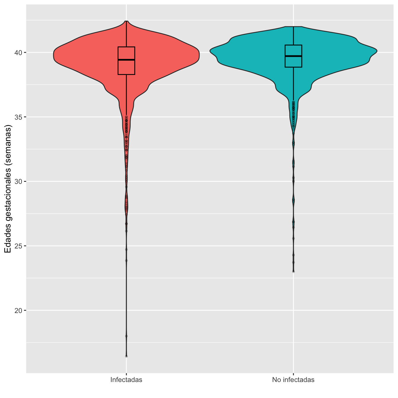
Figura 1.6:
Ajuste de las edades gestacionales de infectadas y no infectadas a distribuciones normales: test de Shapiro-Wilks, p-valores \(8\times 10^{-44}\) y \(2\times 10^{-42}\), respectivamente
Edades gestacionales medias: test t, p-valor \(6\times 10^{-9}\), IC del 95% para la diferencia de medias [-0.57, -0.28]
Desviaciones típicas: test de Fligner-Killeen, p-valor \(2\times 10^{-6}\)
Nota: Como vemos en los boxplot, hay dos casos de infectadas con edades gestacionales incompatibles con la definición de “parto” (y que además luego tienen información incompatible con esto). Son 00133-00046 y 00268-00008. Si las quitamos, las conclusiones son las mismas:
Ajuste de las edades gestacionales de infectadas y no infectadas a distribuciones normales: test de Shapiro-Wilks, p-valores \(3\times 10^{-41}\) y \(2\times 10^{-42}\), respectivamente
Edades medias: test t, p-valor \(2\times 10^{-8}\), IC del 95% para la diferencia de medias [-0.54, -0.26]
Desviaciones típicas: test de Fligner-Killeen, p-valor \(3\times 10^{-6}\)
1.2.9 Prematuridad
| Infectadas (N) | Infectadas (%) | No infectadas (N) | No infectadas (%) | RA | Extr. Inf. IC RA | Extr. Sup. IC RA | RR | Extr. Inf. IC RA | Extr. Sup. IC RR | p-valor | |
|---|---|---|---|---|---|---|---|---|---|---|---|
| Prematuro | 169 | 10.1 | 94 | 5.8 | 0.0428 | 0.0237 | 0.0619 | 1.73 | 1.36 | 2.21 | 6.2e-06 |
| No prematuro | 1499 | 89.9 | 1513 | 94.2 | |||||||
| Datos perdidos | 0 | 0 |
1.2.10 Eventos trombóticos
I=Casos$EVENTOS_TROMBO_TOTALES
NI1=Controls$DVT
NI2=Controls$PE
NI=rep(NA,n_NI)
for (i in 1:n_NI){NI[i]=max(NI1[i],NI2[i],na.rm=TRUE)}
Tabla.DMGC(I,NI,"No eventos trombóticos","Eventos trombóticos")| Infectadas (N) | Infectadas (%) | No infectadas (N) | No infectadas (%) | RA | Extr. Inf. IC RA | Extr. Sup. IC RA | RR | Extr. Inf. IC RA | Extr. Sup. IC RR | p-valor | |
|---|---|---|---|---|---|---|---|---|---|---|---|
| Eventos trombóticos | 12 | 0.7 | 2 | 0.1 | 0.0059 | 9e-04 | 0.011 | 5.78 | 1.45 | 23.05 | 0.013 |
| No eventos trombóticos | 1656 | 99.3 | 1605 | 99.9 | |||||||
| Datos perdidos | 0 | 0 |
1.2.11 Eventos hemorrágicos
I=Casos$EVENTOS_HEMORRAGICOS_TOTAL
NI=Controls$eventos_hemorragicos
Tabla.DMGC(I,NI,"No eventos heomorrágicos","Eventos hemorrágicos")| Infectadas (N) | Infectadas (%) | No infectadas (N) | No infectadas (%) | RA | Extr. Inf. IC RA | Extr. Sup. IC RA | RR | Extr. Inf. IC RA | Extr. Sup. IC RR | p-valor | |
|---|---|---|---|---|---|---|---|---|---|---|---|
| Eventos hemorrágicos | 91 | 5.5 | 89 | 5.5 | -8e-04 | -0.0171 | 0.0154 | 0.99 | 0.74 | 1.31 | 0.939 |
| No eventos heomorrágicos | 1577 | 94.5 | 1518 | 94.5 | |||||||
| Datos perdidos | 0 | 0 |
1.2.12 Ingreso materno en UCI
| Infectadas (N) | Infectadas (%) | No infectadas (N) | No infectadas (%) | RA | Extr. Inf. IC RA | Extr. Sup. IC RA | RR | Extr. Inf. IC RA | Extr. Sup. IC RR | p-valor | |
|---|---|---|---|---|---|---|---|---|---|---|---|
| UCI | 37 | 2.2 | 2 | 0.1 | 0.0209 | 0.0131 | 0.0288 | 17.82 | 4.76 | 66.93 | 0 |
| No UCI | 1631 | 97.8 | 1605 | 99.9 | |||||||
| Datos perdidos | 0 | 0 |
1.2.13 Ingreso materno en UCI según el momento del parto o cesárea
UCI.I=sum(Casos$UCI,na.rm=TRUE)
UCI.NI=sum(Controls$UCI...9,na.rm=TRUE)
I=Casos$UCI_ANTES.DESPUES.DEL.PARTO
NI=Controls$UCI.ANTES.DEL.PARTO  #Vacía
NA_I=length(I[is.na(I)])
NA_NI=length(NI[is.na(NI)])


EE=rbind(as.vector(table(I)),
         c(0,UCI.NI))
FT=fisher.test(EE)
PT=prop.test(EE[,1],rowSums(EE))

RA=round(PT$estimate[1]-PT$estimate[2],3)
ICRA=round(PT$conf.int,4)
RR=round(PT$estimate[1]/PT$estimate[2],2)
ICRR=round(RelRisk(EE,conf.level=0.95,method="score")[2:3],2)

EEExt=rbind(c(as.vector(table(I))[2:1],NA_I),
            c(round(100*as.vector(table(I))[2:1]/(UCI.I-NA_I),1),NA),
            c(as.vector(c(0,UCI.NI))[2:1],NA_NI),
            c(round(100*as.vector(c(0,UCI.NI))[2:1]/(UCI.NI-NA_NI),1),NA),
            c(RA,NA,NA),
            c(ICRA[1],NA,NA),
            c(ICRA[2],NA,NA),
            c(RR,NA,NA),
            c(ICRR[1],NA,NA),
            c(ICRR[2],NA,NA),
            c(round(FT$p.value,4),NA,NA)
            )

colnames(EEExt)=c("Después del parto","Antes del parto" ,"Datos perdidos")
rownames(EEExt)=c("Infectadas (N)", "Infectadas (%)","No infectadas (N)", "No infectadas (%)","RA","Extr. Inf. IC RA","Extr. Sup. IC RA","RR","Extr. Inf. IC RA","Extr. Sup. IC RR", "p-valor")


t(EEExt) %>%
  kbl() %>%
  kable_styling() %>%
scroll_box(width="100%", box_css="border: 0px;")| Infectadas (N) | Infectadas (%) | No infectadas (N) | No infectadas (%) | RA | Extr. Inf. IC RA | Extr. Sup. IC RA | RR | Extr. Inf. IC RA | Extr. Sup. IC RR | p-valor | |
|---|---|---|---|---|---|---|---|---|---|---|---|
| Después del parto | 27 | -1.7 | 2 | -0.1 | 0.27 | -0.1363 | 0.6769 | Inf | 0.35 | Inf | 1 |
| Antes del parto | 10 | -0.6 | 0 | 0.0 | |||||||
| Datos perdidos | 1631 | 1607 |
1.2.14 Embarazos con algún feto muerto anteparto
I=Casos$Feto.muerto.intraútero
I[I=="Sí"]=1
I[I=="No"]=0
NI1=Controls$Feto.vivo...194
NI1[NI1=="Sí"]=0
NI1[NI1=="No"]=1
NI2=Controls$Feto.vivo...245
NI2[NI2=="Sí"]=0
NI2[NI2=="No"]=1
NI=NI1
for (i in 1:length(NI1)){NI[i]=max(NI1[i],NI2[i],na.rm=TRUE)}

Tabla.DMGC(I,NI,"Ningún feto muerto anteparto","Algún feto muerto anteparto")| Infectadas (N) | Infectadas (%) | No infectadas (N) | No infectadas (%) | RA | Extr. Inf. IC RA | Extr. Sup. IC RA | RR | Extr. Inf. IC RA | Extr. Sup. IC RR | p-valor | |
|---|---|---|---|---|---|---|---|---|---|---|---|
| Algún feto muerto anteparto | 19 | 1.1 | 3 | 0.2 | 0.0095 | 0.0034 | 0.0156 | 6.1 | 1.93 | 19.3 | 9e-04 |
| Ningún feto muerto anteparto | 1649 | 98.9 | 1604 | 99.8 | |||||||
| Datos perdidos | 0 | 0 |
1.2.15 Inicio del parto
I=Casos$Inicio.de.parto
I=factor(Casos$Inicio.de.parto,levels=c("Espontáneo", "Inducido", "Cesárea"),ordered=TRUE)
NI=Controls$Inicio.de.parto
NI[NI=="Cesárea programada"]="Cesárea"
NI=factor(NI,levels=c("Espontáneo", "Inducido", "Cesárea"),ordered=TRUE)

Tabla.DMGCm(I,NI,c("Espontáneo", "Inducido", "Cesárea"),r=9)| Infectadas (N) | Infectadas (%) | No infectadas (N) | No infectadas (%) | RA | Extr. Inf. IC RA | Extr. Sup. IC RA | RR | Extr. Inf. IC RA | Extr. Sup. IC RR | p-valor | |
|---|---|---|---|---|---|---|---|---|---|---|---|
| Espontáneo | 871 | 52.3 | 1000 | 62.2 | -0.0995 | -0.1338 | -0.0651 | 0.840 | 0.792 | 0.892 | 0.0000000 |
| Inducido | 628 | 37.7 | 522 | 32.5 | 0.0521 | 0.0189 | 0.0854 | 1.160 | 1.057 | 1.274 | 0.0055636 |
| Cesárea | 167 | 10.0 | 85 | 5.3 | 0.0473 | 0.0286 | 0.0661 | 1.895 | 1.474 | 2.437 | 0.0000011 |
| Datos perdidos | 2 | 0 |
df =data.frame(
  Factor=c( rep("Infectadas",length(I)), rep("No infectadas",length(NI))),
  Inicios=ordered(c( I,NI ),levels=c("Espontáneo","Inducido","Cesárea"))
)

base=ordered(rep(c("Espontáneo","Inducido","Cesárea"), each=2),levels=c("Espontáneo","Inducido","Cesárea"))
Grupo=rep(c("Infectada","No infectada") , 3)
valor=c(as.vector(prop.table(table(df),margin=1))                 )
data <- data.frame(base,Grupo,valor)


ggplot(data, aes(fill=base, y=valor, x=Grupo)) +
  geom_bar(position="dodge", stat="identity")+
  ylab("")+
  scale_fill_brewer(palette = "Set3")+
  labs(fill = "Inicio de parto")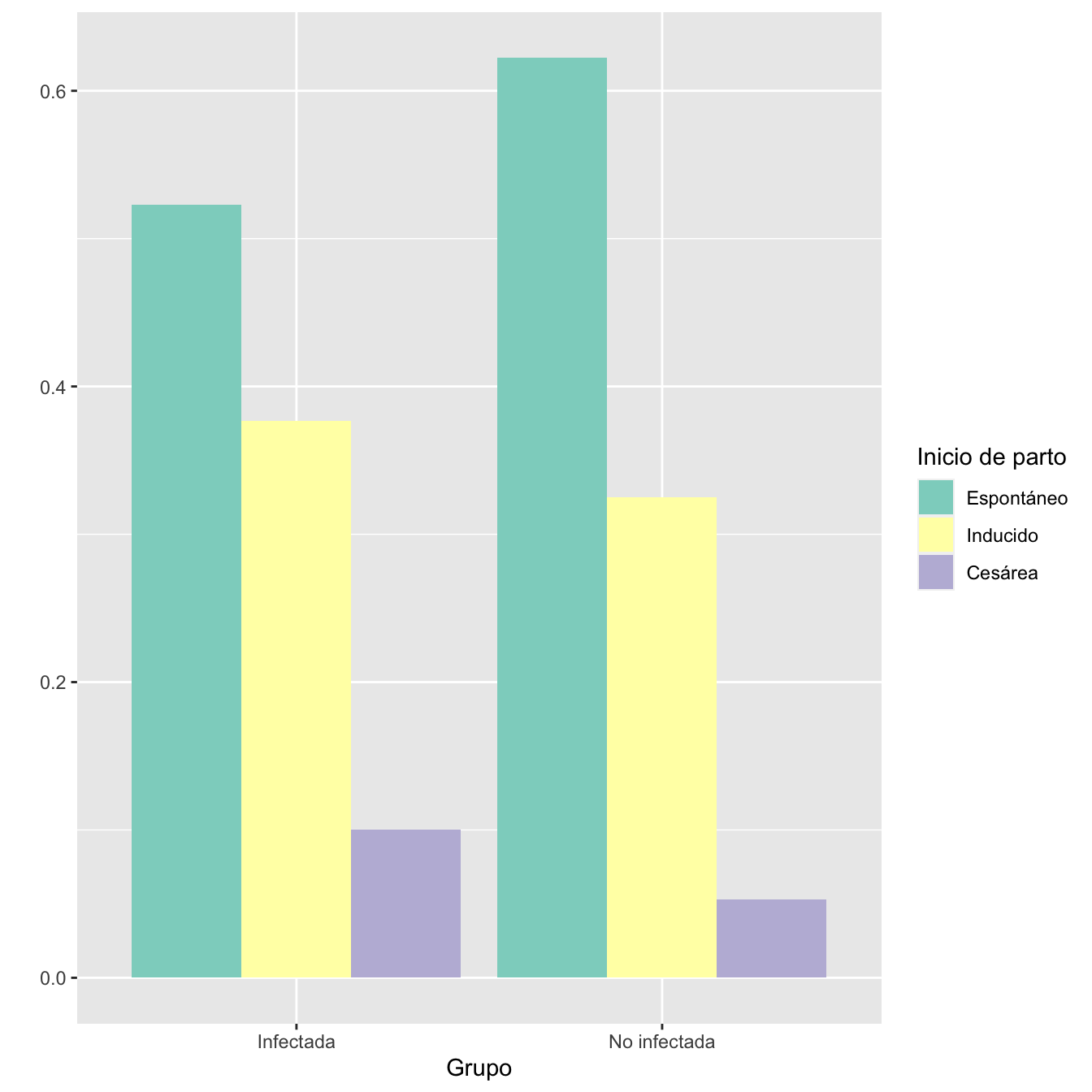
Figura 1.7:
df =data.frame(
  Factor=c( rep("Infectadas",length(I)), rep("No infectadas",length(NI))),
  Inicios=ordered(c( I,NI ),levels=c("Espontáneo","Inducido","Cesárea"))
)

base=ordered(rep(c("Espontáneo","Inducido","Cesárea"), each=2),levels=c("Espontáneo","Inducido","Cesárea"))
Grupo=rep(c("Infectada","No infectada") , 3)
valor=c(as.vector(prop.table(table(df),margin=2))                 )
data <- data.frame(base,Grupo,valor)


ggplot(data, aes(fill=Grupo, y=valor, x=base)) +
  geom_bar(position="dodge", stat="identity")+
  xlab("Inicios de parto")+
  ylab("")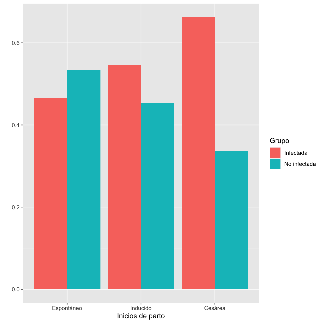
Figura 1.8:
- Distribuciones de los inicios de parto en los grupos de infectadas y no infectadas: test \(\chi^2\), p-valor \(2\times 10^{-10}\)
1.2.16 Tipo de parto
I.In=Casos$Inicio.de.parto
I.In[I.In=="Cesárea"]="Cesárea programada"
I=Casos$Tipo.de.parto
I[I.In=="Cesárea programada"]="Cesárea programada"
I[I=="Cesárea"]="Cesárea urgente"
I[I=="Eutocico"]="Eutócico"
I=factor(I,levels=c("Eutócico", "Instrumental", "Cesárea programada", "Cesárea urgente"),ordered=TRUE)

NI.In=Controls$Inicio.de.parto
NI=Controls$Tipo.de.parto
NI[NI.In=="Cesárea programada"]="Cesárea programada"
NI[NI=="Cesárea"]="Cesárea urgente"
NI[NI=="Eutocico"]="Eutócico"
NI=factor(NI,levels=c("Eutócico", "Instrumental", "Cesárea programada", "Cesárea urgente"),ordered=TRUE)

Tabla.DMGCm(I,NI,c("Eutócico", "Instrumental", "Cesárea programada", "Cesárea urgente"),r=6)| Infectadas (N) | Infectadas (%) | No infectadas (N) | No infectadas (%) | RA | Extr. Inf. IC RA | Extr. Sup. IC RA | RR | Extr. Inf. IC RA | Extr. Sup. IC RR | p-valor | |
|---|---|---|---|---|---|---|---|---|---|---|---|
| Eutócico | 1055 | 63.2 | 1044 | 65.0 | -0.0172 | -0.0506 | 0.0163 | 0.974 | 0.925 | 1.025 | 1.000000 |
| Instrumental | 177 | 10.6 | 235 | 14.6 | -0.0401 | -0.0635 | -0.0168 | 0.726 | 0.605 | 0.871 | 0.002408 |
| Cesárea programada | 167 | 10.0 | 85 | 5.3 | 0.0472 | 0.0285 | 0.0659 | 1.893 | 1.472 | 2.434 | 0.000001 |
| Cesárea urgente | 269 | 16.1 | 243 | 15.1 | 0.0101 | -0.0154 | 0.0355 | 1.067 | 0.910 | 1.251 | 1.000000 |
| Datos perdidos | 0 | 0 |
df =data.frame(
  Factor=c( rep("Infectadas",length(I)), rep("No infectadas",length(NI))),
  Inicios=ordered(c( I,NI ),levels=c("Eutócico", "Instrumental", "Cesárea programada", "Cesárea urgente"))
)

base=ordered(rep(c("Eutócico", "Instrumental", "Cesárea prog.", "Cesárea urg."), each=2),levels=c("Eutócico", "Instrumental", "Cesárea prog.", "Cesárea urg."))
Grupo=rep(c("Infectada","No infectada") , 4)
valor=c(as.vector(prop.table(table(df),margin=1))                 )
data <- data.frame(base,Grupo,valor)


ggplot(data, aes(fill=base, y=valor, x=Grupo)) +
  geom_bar(position="dodge", stat="identity")+
  ylab("")+
  scale_fill_brewer(palette = "Set3")+
  labs(fill = "Tipo de parto")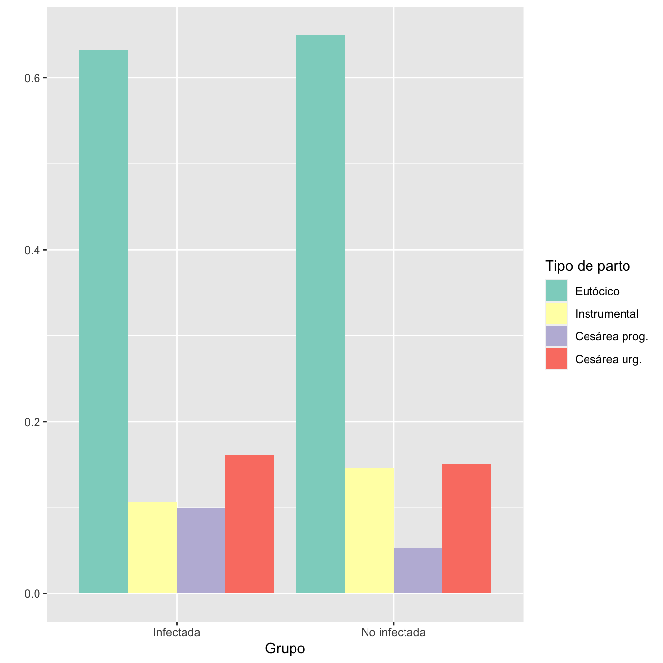
Figura 1.9:
df =data.frame(
  Factor=c( rep("Infectadas",length(I)), rep("No infectadas",length(NI))),
  Inicios=ordered(c( I,NI ),levels=c("Eutócico", "Instrumental", "Cesárea programada", "Cesárea urgente"))
)

base=ordered(rep(c("Eutócico", "Instrumental", "Cesárea prog.", "Cesárea urg."), each=2),levels=c("Eutócico", "Instrumental", "Cesárea prog.", "Cesárea urg."))
Grupo=rep(c("Infectada","No infectada") , 4)
valor=as.vector(prop.table(table(df), margin=2))
data <- data.frame(base,Grupo,valor)


ggplot(data, aes(fill=Grupo, y=valor, x=base)) +
  geom_bar(position="dodge", stat="identity")+
  xlab("Tipos de parto")+
  ylab("")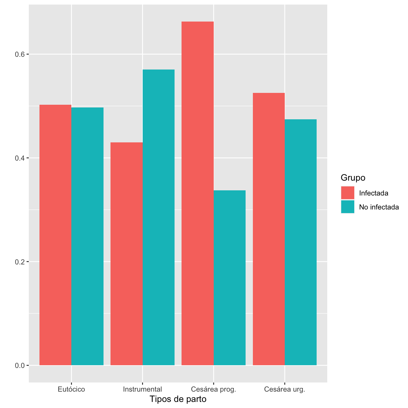
Figura 1.10:
- Distribuciones de los tipos de parto en los grupos de infectadas y no infectadas: test \(\chi^2\), p-valor \(10^{-7}\)
1.2.17 Hemorragias postparto
I=Casos$Hemorragia.postparto
I.sino=I
I.sino[!is.na(I.sino)& I.sino!="No"]="Sí"
I=ordered(I,levels=names(table(I))[c(2,3,1,4)])


NI=Controls$Hemorragia.postparto
NI.sino=NI
NI.sino[!is.na(NI.sino)& NI.sino!="No"]="Sí"
NI=ordered(NI,levels=names(table(NI))[c(2,3,1,4)])

Tabla.DMGC(I.sino,NI.sino,"No HPP","HPP")| Infectadas (N) | Infectadas (%) | No infectadas (N) | No infectadas (%) | RA | Extr. Inf. IC RA | Extr. Sup. IC RA | RR | Extr. Inf. IC RA | Extr. Sup. IC RR | p-valor | |
|---|---|---|---|---|---|---|---|---|---|---|---|
| HPP | 73 | 4.5 | 70 | 4.4 | 5e-04 | -0.0142 | 0.0152 | 1.01 | 0.73 | 1.39 | 1 |
| No HPP | 1561 | 95.5 | 1513 | 95.6 | |||||||
| Datos perdidos | 34 | 24 |
Tabla.DMGCm(I,NI,c("HPP tratamiento médico" ,
"HPP tratamiento quirúrgico conservador",
"Histerectomía obstétrica"    ,
"No") ,r=6)| Infectadas (N) | Infectadas (%) | No infectadas (N) | No infectadas (%) | RA | Extr. Inf. IC RA | Extr. Sup. IC RA | RR | Extr. Inf. IC RA | Extr. Sup. IC RR | p-valor | |
|---|---|---|---|---|---|---|---|---|---|---|---|
| HPP tratamiento médico | 59 | 3.6 | 59 | 3.7 | -0.0012 | -0.0148 | 0.0125 | 0.969 | 0.681 | 1.378 | 1.000000 |
| HPP tratamiento quirúrgico conservador | 9 | 0.6 | 10 | 0.6 | -0.0008 | -0.0067 | 0.0051 | 0.872 | 0.364 | 2.091 | 1.000000 |
| Histerectomía obstétrica | 5 | 0.3 | 1 | 0.1 | 0.0024 | -0.0011 | 0.0060 | 4.844 | 0.797 | 29.423 | 0.874665 |
| No | 1561 | 95.5 | 1513 | 95.6 | -0.0005 | -0.0152 | 0.0142 | 1.000 | 0.985 | 1.014 | 1.000000 |
| Datos perdidos | 34 | 24 |
df =data.frame(
  Factor=c( rep("Infectadas",length(I[I!="No"])), rep("No infectadas",length(NI[NI!="No"]))),
  Hemos=ordered(c( I[I!="No"],NI[NI!="No"] ),levels=names(table(I))[-4])
)

base=ordered(rep(c("Tto. médico", "Tto. Qx conservador", "Histerectomía"), each=2),levels=c("Tto. médico", "Tto. Qx conservador", "Histerectomía"))
Grupo=rep(c("Infectada","No infectada") , 3)
valor=as.vector(prop.table(table(df), margin=1))
data <- data.frame(base,Grupo,valor)


ggplot(data, aes(fill=Grupo, y=valor, x=base)) +
  geom_bar(position="dodge", stat="identity")+
  xlab("Tratamientos de hemorragia postparto")+
  ylab("")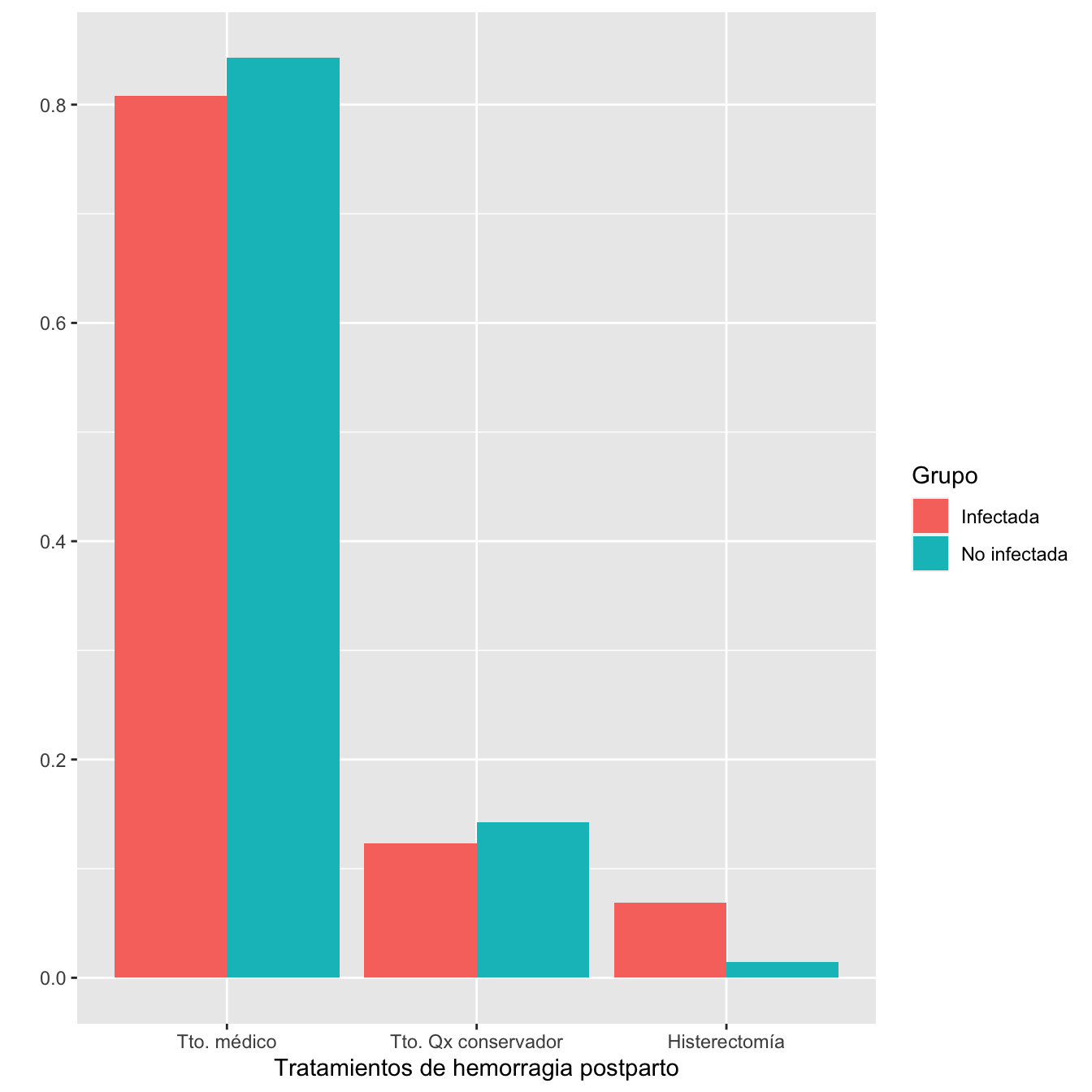
Figura 1.11:
Distribuciones de los tipos de hemorragia postparto (incluyendo Noes) en los grupos de infectadas y no infectadas: test \(\chi^2\) de Montercarlo, p-valor 0.47
Distribuciones de los tipos de hemorragia postparto en los grupos de infectadas y no infectadas que tuvieron hemorragia postparto: test \(\chi^2\) de Montercarlo, p-valor 0.61
1.2.18 Fetos muertos anteparto
I1=Casos$Feto.muerto.intraútero
I1[I1=="Sí"]="Muerto"
I1[I1=="No"]="Vivo"
I2=CasosGM$Feto.vivo
I2[I2=="Sí"]="Vivo"
I2[I2=="No"]="Muerto"
I=c(I1,I2)
I=ordered(I,levels=c("Vivo","Muerto"))


n_IFT=length(I)
n_VI=as.vector(table(I))[1]NI1=Controls$Feto.vivo...194
NI2=ControlsGM$Feto.vivo...245
NI=c(NI1,NI2)
NI[NI=="Sí"]="Vivo"
NI[NI=="No"]="Muerto"
NI=ordered(NI,levels=c("Vivo","Muerto"))
n_NIFT=length(NI)
n_VNI=as.vector(table(NI))[1]
Tabla.DMGC(I,NI,"Feto vivo","Feto muerto anteparto")| Infectadas (N) | Infectadas (%) | No infectadas (N) | No infectadas (%) | RA | Extr. Inf. IC RA | Extr. Sup. IC RA | RR | Extr. Inf. IC RA | Extr. Sup. IC RR | p-valor | |
|---|---|---|---|---|---|---|---|---|---|---|---|
| Feto muerto anteparto | 19 | 1.1 | 3 | 0.2 | 0.0094 | 0.0033 | 0.0154 | 6.11 | 1.94 | 19.34 | 9e-04 |
| Feto vivo | 1679 | 98.9 | 1636 | 99.8 | |||||||
| Datos perdidos | 1 | 2 |
1.2.19 Peso de neonatos al nacimiento
I=c(Casos[Casos$Feto.muerto.intraútero=="No",]$Peso._gramos_...125,CasosGM[CasosGM$Feto.vivo=="Sí",]$Peso._gramos_...148)
NI=c(Controls[Controls$Feto.vivo...194=="Sí",]$Peso._gramos_...198,ControlsGM[ControlsGM$Feto.vivo...245=="Sí",]$Peso._gramos_...247)
data =data.frame(
name=c(rep("Hijos de infectadas",length(I)), rep("Hijos de no infectadas",length(NI))),
Pesos=c(I,NI)
)
sample_size = data %>% group_by(name) %>% summarize(num=n())
data %>%
left_join(sample_size) %>%
mutate(myaxis = paste0(name, "\n", "n=", num)) %>%
ggplot( aes(x=myaxis, y=Pesos, fill=name)) +
geom_violin(width=0.9) +
geom_boxplot(width=0.1, color="black", alpha=0.2,outlier.fill="black",
outlier.size=1) +
theme(
legend.position="none",
plot.title = element_text(size=11)
) +
xlab("")+
ylab("Pesos (gramos)")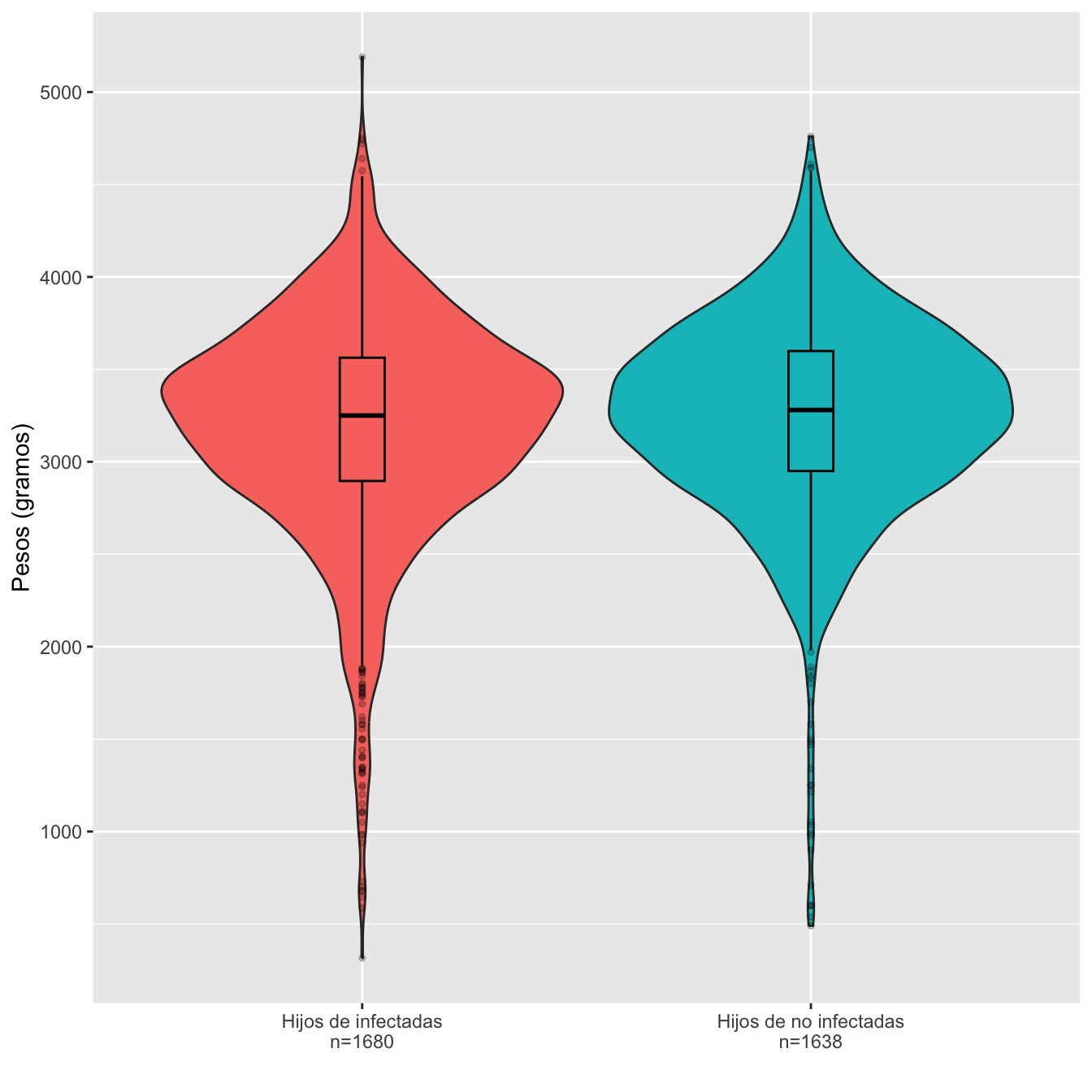
Figura 1.12:
Dades=rbind(c(min(I,na.rm=TRUE),max(I,na.rm=TRUE), round(mean(I,na.rm=TRUE),1),round(median(I,na.rm=TRUE),1),round(quantile(I,c(0.25,0.75),na.rm=TRUE),1), round(sd(I,na.rm=TRUE),1)),
            c(min(NI,na.rm=TRUE),max(NI,na.rm=TRUE), round(mean(NI,na.rm=TRUE),1),round(median(NI,na.rm=TRUE),1),round(quantile(NI,c(0.25,0.75),na.rm=TRUE),1),round(sd(NI,na.rm=TRUE),1)))

colnames(Dades)=c("Peso mínimo","Peso máximo","Peso medio", "Peso mediano", "1er cuartil", "3er cuartil", "Desv. típica")
rownames(Dades)=c("Infectadas", "No infectadas")

Dades %>%
  kbl() %>%
  kable_styling() %>%
scroll_box(width="100%", box_css="border: 0px;")| Peso mínimo | Peso máximo | Peso medio | Peso mediano | 1er cuartil | 3er cuartil | Desv. típica | |
|---|---|---|---|---|---|---|---|
| Infectadas | 315 | 5190 | 3191.0 | 3250 | 2896.2 | 3563 | 603.4 |
| No infectadas | 490 | 4760 | 3248.7 | 3280 | 2950.0 | 3599 | 538.1 |
Ajuste de los pesos de hijos de infectadas y no infectadas a distribuciones normales: test de Shapiro-Wilks, p-valores \(10^{-21}\) y \(2\times 10^{-20}\), respectivamente
Pesos medios: test t, p-valor 0.004, IC del 95% para la diferencia de medias [-96.92, -18.44]
Desviaciones típicas: test de Fligner-Killeen, p-valor 0.0052
Definimos bajo peso a peso menor o igual a 2500 g. Un 8.74% del total de neonatos no muesrtos anteparto son de bajo peso con esta definición.
I.cut=cut(I,breaks=c(0,2500,10000),labels=c(1,0),right=FALSE)
I.cut=ordered(I.cut,levels=c(0,1))
NI.cut=cut(NI,breaks=c(0,2500,10000),labels=c(1,0),right=FALSE)
NI.cut=ordered(NI.cut,levels=c(0,1))

Tabla.DMGC(I.cut,NI.cut,"No bajo peso","Bajo peso")| Infectadas (N) | Infectadas (%) | No infectadas (N) | No infectadas (%) | RA | Extr. Inf. IC RA | Extr. Sup. IC RA | RR | Extr. Inf. IC RA | Extr. Sup. IC RR | p-valor | |
|---|---|---|---|---|---|---|---|---|---|---|---|
| Bajo peso | 172 | 10.5 | 113 | 7 | 0.035 | 0.015 | 0.0549 | 1.5 | 1.2 | 1.88 | 4e-04 |
| No bajo peso | 1470 | 89.5 | 1506 | 93 | |||||||
| Datos perdidos | 38 | 19 |
1.2.20 Apgar
I=c(Casos$APGAR.5...126,CasosGM$APGAR.5...150)
I[I==19]=NA
NI=c(Controls$APGAR.5...200,ControlsGM$APGAR.5...249)

I.5=cut(I,breaks=c(-1,7,20),labels=c("0-7","8-10"))
NI.5=cut(NI,breaks=c(-1,7,20),labels=c("0-7","8-10"))
I.5=ordered(I.5,levels=c("8-10","0-7"))
NI.5=ordered(NI.5,levels=c("8-10","0-7"))

Tabla.DMGC(I.5,NI.5,"Apgar.5≥8","Apgar.5≤7")| Infectadas (N) | Infectadas (%) | No infectadas (N) | No infectadas (%) | RA | Extr. Inf. IC RA | Extr. Sup. IC RA | RR | Extr. Inf. IC RA | Extr. Sup. IC RR | p-valor | |
|---|---|---|---|---|---|---|---|---|---|---|---|
| Apgar.5≤7 | 50 | 3 | 33 | 2 | 0.0096 | -0.0017 | 0.0208 | 1.47 | 0.96 | 2.27 | 0.0949 |
| Apgar.5≥8 | 1627 | 97 | 1596 | 98 | |||||||
| Datos perdidos | 22 | 12 |
1.2.21 Ingreso de neonatos vivos en UCIN
I=c(Casos[Casos$Feto.muerto.intraútero=="No",]$Ingreso.en.UCIN,CasosGM[CasosGM$Feto.vivo=="Sí",]$Ingreso.en.UCI)
NI=c(Controls[Controls$Feto.vivo...194=="Sí",]$Ingreso.en.UCI...213,ControlsGM[ControlsGM$Feto.vivo...245=="Sí",]$Ingreso.en.UCI...260)

Tabla.DMGC(I,NI,"No UCIN","UCIN")| Infectadas (N) | Infectadas (%) | No infectadas (N) | No infectadas (%) | RA | Extr. Inf. IC RA | Extr. Sup. IC RA | RR | Extr. Inf. IC RA | Extr. Sup. IC RR | p-valor | |
|---|---|---|---|---|---|---|---|---|---|---|---|
| UCIN | 157 | 9.5 | 42 | 2.6 | 0.0689 | 0.0522 | 0.0855 | 3.67 | 2.63 | 5.12 | 0 |
| No UCIN | 1501 | 90.5 | 1585 | 97.4 | |||||||
| Datos perdidos | 22 | 11 |
1.2.22 Otros
1.2.22.1 Relación entre cesárea y obesidad en infectadas
##
##  Fisher's Exact Test for Count Data
##
## data:  EE
## p-value = 7.028e-05
## alternative hypothesis: true odds ratio is not equal to 1
## 95 percent confidence interval:
##  1.312108 2.272104
## sample estimates:
## odds ratio
## 1.729206PT=prop.test(EE[,1],rowSums(EE))
RA=round(PT$estimate[1]-PT$estimate[2],4)
ICRA=round(PT$conf.int,4)
RR=round(PT$estimate[1]/PT$estimate[2],2)
ICRR=round(RelRisk(EE,conf.level=0.95,method="score")[2:3],2)- RA: 0.1135, IC 95% 0.0532, 0.1737
- RR: 1.47, IC 95% 1.23, 1.75