Lección 3 Descripción global de la muestra de la primera ola
Casos=Casos1w
Controls=Controls1w
Sint=Casos$SINTOMAS_DIAGNOSTICO
CasosGM=Casos1wGM
ControlsGM=Controls1wGM
Hay 877 infectadas y 1191 no infectadas en la muestra de la primera ola.
3.1 Antecedentes
3.1.1 Edades
data =data.frame(
  name=c(rep("Infectadas",length(I)), rep("No infectadas",length(NI))),
  Edades=c(I,NI)
  )

sample_size = data %>% group_by(name) %>% summarize(num=n())

data %>%
 left_join(sample_size) %>%
  mutate(myaxis = paste0(name, "\n", "n=", num)) %>%
  ggplot( aes(x=myaxis, y=Edades, fill=name)) +
    geom_violin(width=1) +
    geom_boxplot(width=0.1, color="black", alpha=0.2,outlier.fill="black",
               outlier.size=1) +
    theme(
      legend.position="none",
      plot.title = element_text(size=11)
    ) +
    xlab("")+
  ylab("Edades (años)")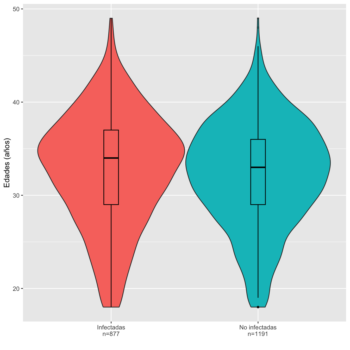
Figura 3.1:
Dades=rbind(c(min(I,na.rm=TRUE),max(I,na.rm=TRUE), round(mean(I,na.rm=TRUE),1),round(median(I,na.rm=TRUE),1),round(quantile(I,c(0.25,0.75),na.rm=TRUE),1), round(sd(I,na.rm=TRUE),1)),
            c(min(NI,na.rm=TRUE),max(NI,na.rm=TRUE), round(mean(NI,na.rm=TRUE),1),round(median(NI,na.rm=TRUE),1),round(quantile(NI,c(0.25,0.75),na.rm=TRUE),1),round(sd(NI,na.rm=TRUE),1)))

colnames(Dades)=c("Edad mínima","Edad máxima","Edad media", "Edad mediana", "1er cuartil", "3er cuartil", "Desv. típica")
rownames(Dades)=c("Infectadas", "No infectadas")

Dades %>%
  kbl() %>%
  kable_styling() %>%
scroll_box(width="100%", box_css="border: 0px;")| Edad mínima | Edad máxima | Edad media | Edad mediana | 1er cuartil | 3er cuartil | Desv. típica | |
|---|---|---|---|---|---|---|---|
| Infectadas | 18 | 49 | 32.7 | 34 | 29 | 37 | 6.0 |
| No infectadas | 18 | 49 | 32.3 | 33 | 29 | 36 | 5.7 |
Ajuste de las edades de infectadas y no infectadas a distribuciones normales: test de Shapiro-Wilks, p-valores \(8\times 10^{-8}\) y \(3\times 10^{-8}\), respectivamente
Igualdad de edades medias: test t, p-valor 0.08, IC del 95% para la diferencia de medias [-0.06, 0.97] años
Igualdad de desviaciones típicas: test de Fligner-Killeen, p-valor \(0.05696\)
En las tablas como la que sigue:
- Los porcentajes se han calculado en la muestra sin pérdidas
- OR: la odds ratio univariante estimada de infectarse relativa a la franja de edad
- IC: el intervalo de confianza del 95% para la OR
- p-valor ajustado: p-valores de tests de Fisher bilaterales ajustados por Bonferroni calculados para la muestra sin pérdidas
I.cut=cut(I,breaks=c(0,30,40,100),labels=c("18-30","31-40",">40"))
NI.cut=cut(NI,breaks=c(0,30,40,100),labels=c("18-30","31-40",">40"))
Tabla.DMGm(I.cut,NI.cut,c("18-30","31-40",">40"))| Infectadas (N) | Infectadas (%) | No infectadas (N) | No infectadas (%) | OR | Extr. Inf. IC | Extr. Sup. IC | p-valor ajustado | |
|---|---|---|---|---|---|---|---|---|
| 18-30 | 286 | 32.8 | 416 | 35.3 | 0.89 | 0.74 | 1.08 | 0.7575 |
| 31-40 | 516 | 59.1 | 695 | 58.9 | 1.01 | 0.84 | 1.21 | 1.0000 |
| >40 | 71 | 8.1 | 68 | 5.8 | 1.45 | 1.01 | 2.07 | 0.1304 |
| Datos perdidos | 4 | 12 |
df =data.frame(
  Factor=c(rep("Infectadas",length(I)), rep("No infectadas",length(NI))),
  Edades=c( I.cut,NI.cut )
)

base=ordered(rep(c("18-30","31-40",">40"), each=2),levels=c("18-30", "31-40",   ">40"))
Grupo=rep(c("Infectada","No infectada") , length(levels(I.cut)))
valor=as.vector(prop.table(table(df), margin=1))
data <- data.frame(base,Grupo,valor)


ggplot(data, aes(fill=base , y=valor, x=Grupo)) +
  geom_bar(position="dodge", stat="identity")+
  ylab("")+
  scale_fill_brewer(palette = "Accent")+
  labs(fill = "Grupo de edad")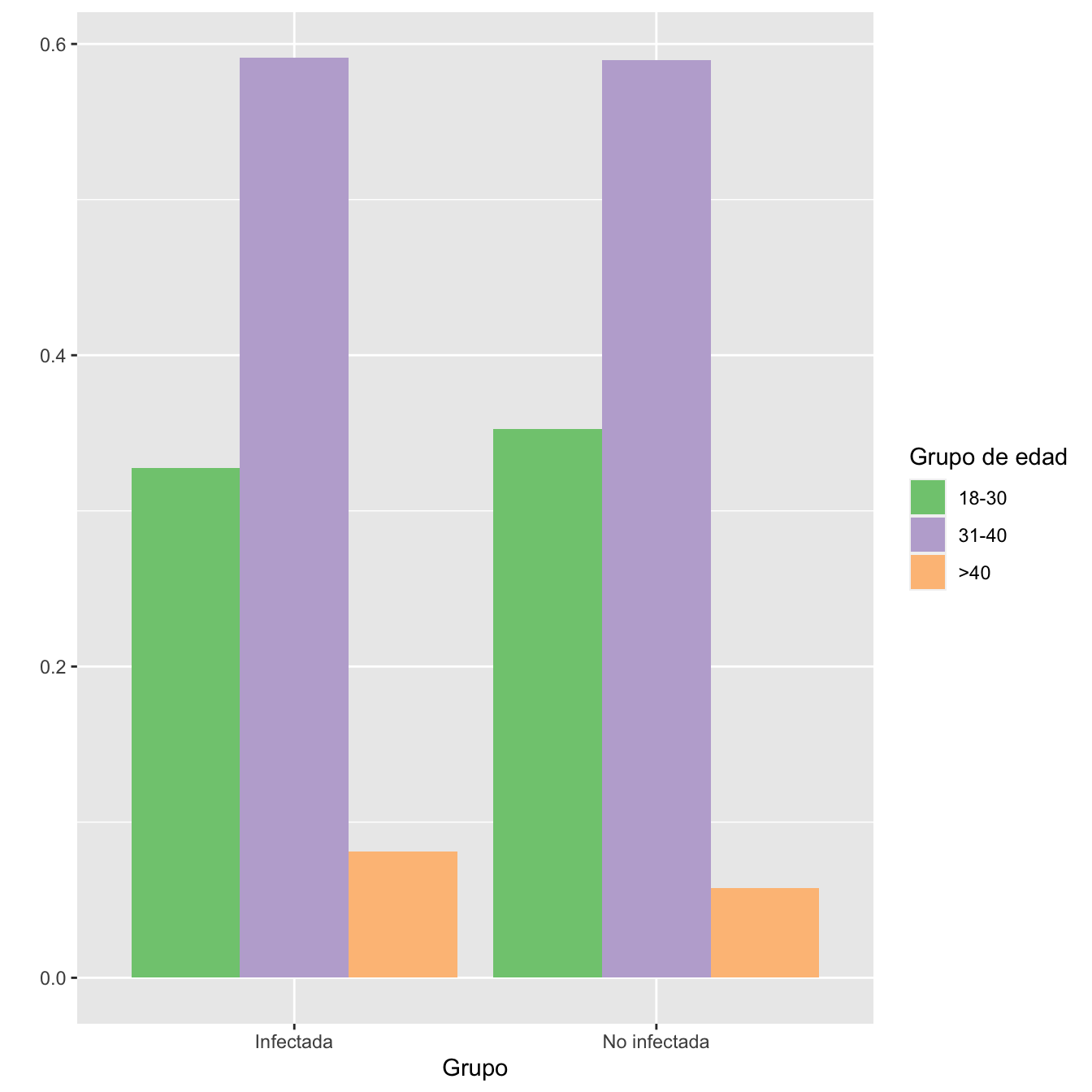
Figura 3.2:
df =data.frame(
  Factor=c(rep("Infectadas",length(I)), rep("No infectadas",length(NI))),
  Edades=c( I.cut,NI.cut )
)

base=ordered(rep(c("18-30","31-40",">40"), each=2),levels=c("18-30", "31-40",   ">40"))
Grupo=rep(c("Infectada","No infectada") , length(levels(I.cut)))
valor=as.vector(prop.table(table(df), margin=2))
data <- data.frame(base,Grupo,valor)


ggplot(data, aes(fill=Grupo, y=valor, x=base)) +
  geom_bar(position="dodge", stat="identity")+
xlab("Grupos de edad")+
  ylab("")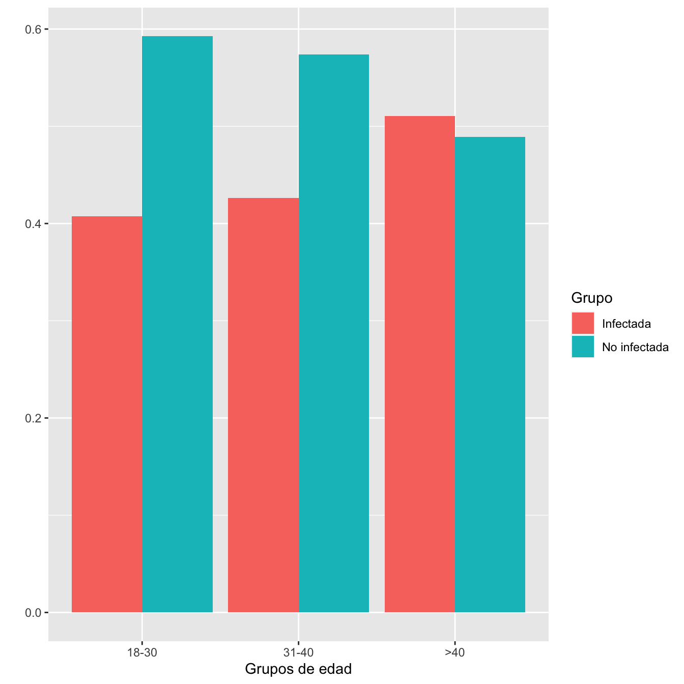
Figura 3.3:
- Igualdad de composiciones por edades de los grupos de casos y de controles: test \(\chi^2\), p-valor 0.0789.
3.1.2 Etnias
I=Casos$Etnia
I[I=="Asia"]="Asiática"
I=factor(I)
NI=factor(Controls$Etnia)
Tabla.DMGm(I,NI,c("Árabe", "Asiática", "Blanca", "Latinoamericana","Negra"),r=6)| Infectadas (N) | Infectadas (%) | No infectadas (N) | No infectadas (%) | OR | Extr. Inf. IC | Extr. Sup. IC | p-valor ajustado | |
|---|---|---|---|---|---|---|---|---|
| Árabe | 54 | 6.2 | 108 | 9.1 | 0.66 | 0.46 | 0.93 | 0.093463 |
| Asiática | 24 | 2.7 | 27 | 2.3 | 1.21 | 0.66 | 2.20 | 1.000000 |
| Blanca | 537 | 61.4 | 922 | 77.7 | 0.46 | 0.38 | 0.56 | 0.000000 |
| Latinoamericana | 240 | 27.5 | 114 | 9.6 | 3.56 | 2.78 | 4.59 | 0.000000 |
| Negra | 19 | 2.2 | 16 | 1.3 | 1.63 | 0.79 | 3.40 | 1.000000 |
| Datos perdidos | 3 | 4 |
df =data.frame(
  Factor=c(rep("Infectadas",length(I)), rep("No infectadas",length(NI))),
  Etnias=c(I,NI)
)
base=rep(levels(I) , each=2)
Grupo=rep(c("Infectada","No infectada") , length(levels(I)))
valor=as.vector(prop.table(table(df), margin=1))
data <- data.frame(base,Grupo,valor)


ggplot(data, aes(fill=base , y=valor, x=Grupo)) +
  geom_bar(position="dodge", stat="identity")+
  ylab("")+
  scale_fill_brewer(palette = "Accent")+
  labs(fill = "Etnia")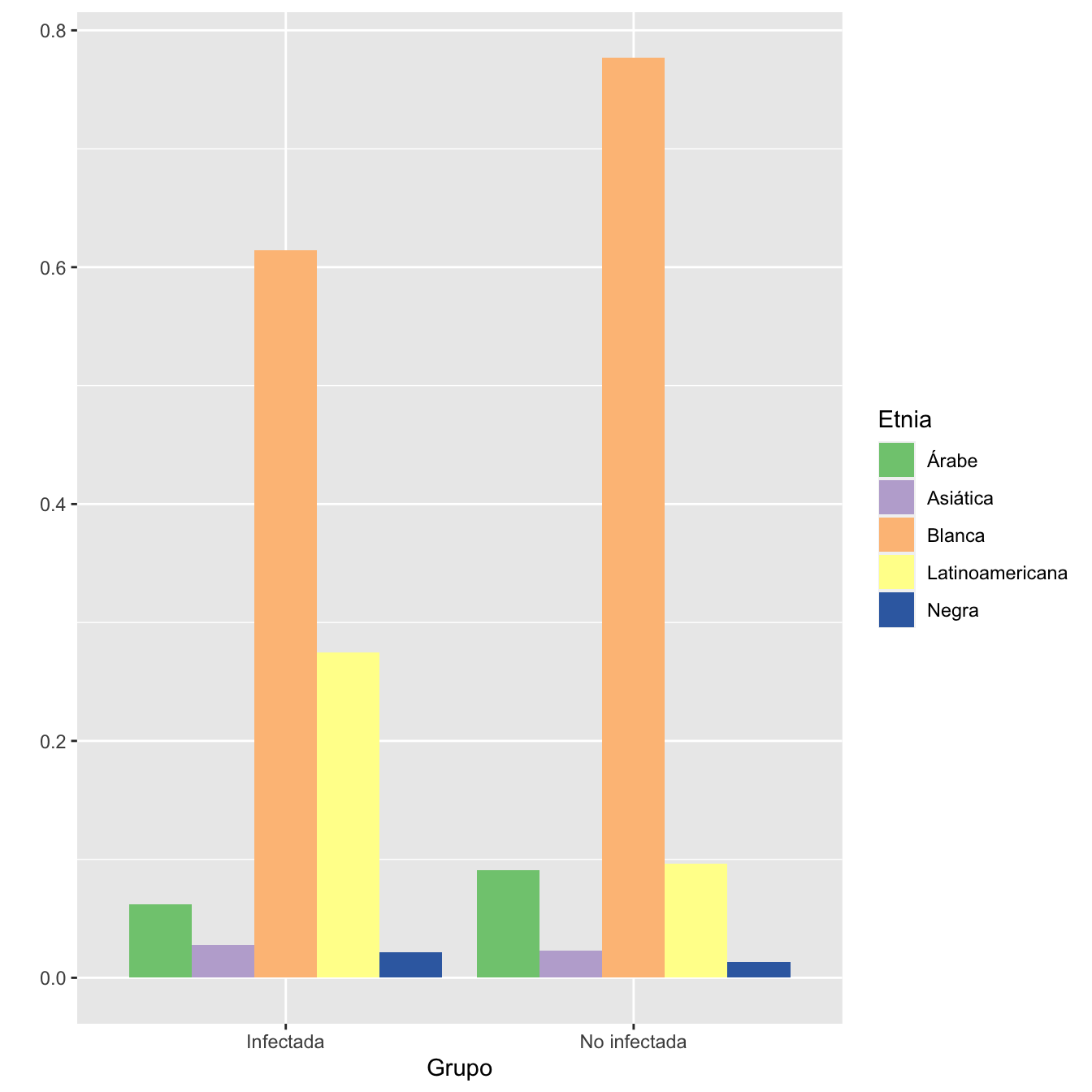
Figura 3.4:
df =data.frame(
  Factor=c(rep("Infectadas",length(I)), rep("No infectadas",length(NI))),
  Etnias=c(I,NI)
)
base=rep(levels(I) , each=2)
Grupo=rep(c("Infectada","No infectada") , length(levels(I)))
valor=as.vector(prop.table(table(df), margin=2))
data <- data.frame(base,Grupo,valor)


ggplot(data, aes(fill=Grupo, y=valor, x=base)) +
  geom_bar(position="dodge", stat="identity")+
xlab("Etnias")+
  ylab("")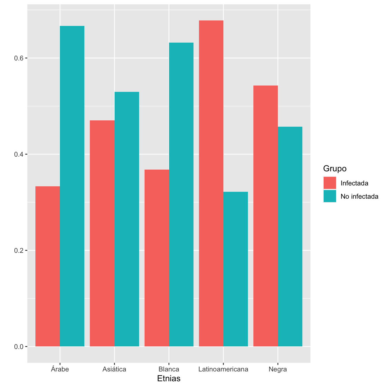
Figura 3.5:
- Composiciones por etnias de los grupos de casos y de controles: test \(\chi^2\), p-valor \(5\times 10^{-25}\)
3.1.3 Hábito tabáquico (juntando fumadoras y ex-fumadoras en una sola categoría)
En las tablas como la que sigue (para antecedentes):
- Los porcentajes se calculan para la muestra sin pérdidas
- La OR es la de infección relativa al antecedente
- El IC es el IC 95% para la OR
- El p-valor es el del test de Fisher bilateral sin tener en cuenta los datos perdidos
| Infectadas (N) | Infectadas (%) | No infectadas (N) | No infectadas (%) | OR | Extr. Inf. IC | Extr. Sup. IC | p-valor | |
|---|---|---|---|---|---|---|---|---|
| Fumadora | 96 | 11.4 | 144 | 12.9 | 0.88 | 0.66 | 1.16 | 0.3657 |
| No fumadora | 743 | 88.6 | 976 | 87.1 | ||||
| Datos perdidos | 38 | 71 |
3.1.4 Obesidad
| Infectadas (N) | Infectadas (%) | No infectadas (N) | No infectadas (%) | OR | Extr. Inf. IC | Extr. Sup. IC | p-valor | |
|---|---|---|---|---|---|---|---|---|
| Obesa | 161 | 18.4 | 198 | 17.5 | 1.06 | 0.84 | 1.34 | 0.6386 |
| No obesa | 716 | 81.6 | 935 | 82.5 | ||||
| Datos perdidos | 0 | 58 |
3.1.5 Hipertensión pregestacional
I=Casos$Hipertensión.pregestacional
NI=Controls$Hipertensión.pregestacional
Tabla.DMG(I,NI,"No HTA","HTA")| Infectadas (N) | Infectadas (%) | No infectadas (N) | No infectadas (%) | OR | Extr. Inf. IC | Extr. Sup. IC | p-valor | |
|---|---|---|---|---|---|---|---|---|
| HTA | 14 | 1.6 | 13 | 1.1 | 1.4 | 0.61 | 3.26 | 0.4366 |
| No HTA | 863 | 98.4 | 1123 | 98.9 | ||||
| Datos perdidos | 0 | 55 |
3.1.6 Diabetes Mellitus
| Infectadas (N) | Infectadas (%) | No infectadas (N) | No infectadas (%) | OR | Extr. Inf. IC | Extr. Sup. IC | p-valor | |
|---|---|---|---|---|---|---|---|---|
| DM | 14 | 1.6 | 17 | 1.4 | 1.12 | 0.51 | 2.43 | 0.8551 |
| No DM | 863 | 98.4 | 1174 | 98.6 | ||||
| Datos perdidos | 0 | 0 |
3.1.7 Enfermedades cardíacas crónicas
| Infectadas (N) | Infectadas (%) | No infectadas (N) | No infectadas (%) | OR | Extr. Inf. IC | Extr. Sup. IC | p-valor | |
|---|---|---|---|---|---|---|---|---|
| ECC | 11 | 1.3 | 21 | 1.8 | 0.69 | 0.3 | 1.5 | 0.3704 |
| No ECC | 866 | 98.7 | 1134 | 98.2 | ||||
| Datos perdidos | 0 | 36 |
3.1.8 Enfermedades pulmonares crónicas (incluyendo asma)
INA=Casos$Enfermedad.pulmonar.crónica.no.asma
NINA=Controls$Enfermedad.pulmonar.crónica.no.asma
NINA[NINA==0]="No"
NINA[NINA==1]="Sí"
IA=Casos$Diagnóstico.clínico.de.Asma
NIA=Controls$Diagnóstico.clínico.de.Asma
NIA[NIA==0]="No"
NIA[NIA==1]="Sí"

I=rep(NA,n_I)
for (i in 1:n_I){I[i]=max(INA[i],IA[i],na.rm=TRUE)}
NI=rep(NA,n_NI)
for (i in 1:n_NI){NI[i]=max(NINA[i],NIA[i],na.rm=TRUE)}
NI[NI==-Inf]=NA


Tabla.DMG(I,NI,"No EPC","EPC")| Infectadas (N) | Infectadas (%) | No infectadas (N) | No infectadas (%) | OR | Extr. Inf. IC | Extr. Sup. IC | p-valor | |
|---|---|---|---|---|---|---|---|---|
| EPC | 38 | 4.3 | 42 | 3.6 | 1.2 | 0.74 | 1.92 | 0.4899 |
| No EPC | 839 | 95.7 | 1111 | 96.4 | ||||
| Datos perdidos | 791 | 454 |
3.1.9 Paridad
| Infectadas (N) | Infectadas (%) | No infectadas (N) | No infectadas (%) | OR | Extr. Inf. IC | Extr. Sup. IC | p-valor | |
|---|---|---|---|---|---|---|---|---|
| Nulípara | 319 | 37 | 451 | 38.1 | 0.95 | 0.79 | 1.15 | 0.6114 |
| Multípara | 544 | 63 | 732 | 61.9 | ||||
| Datos perdidos | 14 | 8 |
3.1.10 Gestación múltiple
I=Casos$Gestación.Múltiple
NI=Controls$Gestación.Múltiple
Tabla.DMG(I,NI,"Gestación única","Gestación múltiple")| Infectadas (N) | Infectadas (%) | No infectadas (N) | No infectadas (%) | OR | Extr. Inf. IC | Extr. Sup. IC | p-valor | |
|---|---|---|---|---|---|---|---|---|
| Gestación múltiple | 18 | 2.1 | 28 | 2.4 | 0.87 | 0.45 | 1.64 | 0.7632 |
| Gestación única | 859 | 97.9 | 1163 | 97.6 | ||||
| Datos perdidos | 0 | 0 |
3.2 Desenlaces
3.2.1 Anomalías congénitas
En las tablas como la que sigue (para desenlaces):
- Los porcentajes se calculan para la muestra sin pérdidas
- RA y RR: riesgo absoluto y relativo del desenlace relativo a la infección
- Los IC son el IC 95% para RA y RR
- El p-valor es el del test de Fisher bilateral sin tener en cuenta los datos perdidos
I=Casos$Diagnóstico.de.malformación.ecográfica._.semana.20._
NI=Controls$Diagnóstico.de.malformación.ecográfica._.semana.20._
Tabla.DMGC(I,NI,"No anomalía congénita","Anomalía congénita")| Infectadas (N) | Infectadas (%) | No infectadas (N) | No infectadas (%) | RA | Extr. Inf. IC RA | Extr. Sup. IC RA | RR | Extr. Inf. IC RA | Extr. Sup. IC RR | p-valor | |
|---|---|---|---|---|---|---|---|---|---|---|---|
| Anomalía congénita | 14 | 1.6 | 12 | 1 | 0.0063 | -0.0051 | 0.0176 | 1.61 | 0.76 | 3.41 | 0.2346 |
| No anomalía congénita | 835 | 98.4 | 1161 | 99 | |||||||
| Datos perdidos | 28 | 18 |
3.2.2 Retraso del crecimiento intrauterino
I=Casos$Defecto.del.crecimiento.fetal..en.tercer.trimestre._.CIR._.
NI=Controls$Defecto.del.crecimiento.fetal..en.tercer.trimestre._.CIR._.
Tabla.DMGC(I,NI,"No RCIU","RCIU")| Infectadas (N) | Infectadas (%) | No infectadas (N) | No infectadas (%) | RA | Extr. Inf. IC RA | Extr. Sup. IC RA | RR | Extr. Inf. IC RA | Extr. Sup. IC RR | p-valor | |
|---|---|---|---|---|---|---|---|---|---|---|---|
| RCIU | 32 | 3.6 | 33 | 2.9 | 0.0079 | -0.0088 | 0.0246 | 1.28 | 0.8 | 2.05 | 0.3124 |
| No RCIU | 845 | 96.4 | 1123 | 97.1 | |||||||
| Datos perdidos | 0 | 35 |
3.2.3 Diabetes gestacional
| Infectadas (N) | Infectadas (%) | No infectadas (N) | No infectadas (%) | RA | Extr. Inf. IC RA | Extr. Sup. IC RA | RR | Extr. Inf. IC RA | Extr. Sup. IC RR | p-valor | |
|---|---|---|---|---|---|---|---|---|---|---|---|
| DG | 66 | 7.5 | 95 | 8.1 | -0.0057 | -0.0301 | 0.0187 | 0.93 | 0.69 | 1.26 | 0.6785 |
| No DG | 811 | 92.5 | 1079 | 91.9 | |||||||
| Datos perdidos | 0 | 17 |
3.2.4 Hipertensión gestacional
| Infectadas (N) | Infectadas (%) | No infectadas (N) | No infectadas (%) | RA | Extr. Inf. IC RA | Extr. Sup. IC RA | RR | Extr. Inf. IC RA | Extr. Sup. IC RR | p-valor | |
|---|---|---|---|---|---|---|---|---|---|---|---|
| HG | 20 | 2.3 | 29 | 2.5 | -0.0019 | -0.0161 | 0.0124 | 0.92 | 0.53 | 1.61 | 0.8841 |
| No HG | 857 | 97.7 | 1146 | 97.5 | |||||||
| Datos perdidos | 0 | 16 |
3.2.5 Preeclampsia
| Infectadas (N) | Infectadas (%) | No infectadas (N) | No infectadas (%) | RA | Extr. Inf. IC RA | Extr. Sup. IC RA | RR | Extr. Inf. IC RA | Extr. Sup. IC RR | p-valor | |
|---|---|---|---|---|---|---|---|---|---|---|---|
| PE | 46 | 5.2 | 56 | 4.7 | 0.0054 | -0.0146 | 0.0255 | 1.12 | 0.76 | 1.63 | 0.6079 |
| No PE | 831 | 94.8 | 1135 | 95.3 | |||||||
| Datos perdidos | 0 | 0 |
3.2.6 Preeclampsia con criterios de gravedad
n_PI=sum(Casos$PREECLAMPSIA_ECLAMPSIA_TOTAL)
n_PNI=sum(Controls$PREECLAMPSIA)
I=Casos[Casos$PREECLAMPSIA_ECLAMPSIA_TOTAL==1,]$Preeclampsia.grave_HELLP_ECLAMPSIA

NI1=Controls[Controls$PREECLAMPSIA==1,]$preeclampsia_severa
NI2=Controls[Controls$PREECLAMPSIA==1,]$Preeclampsia.grave.No.HELLP
NI=rep(NA,n_PNI)
for (i in 1:n_PNI){NI[i]=max(NI1[i],NI2[i],na.rm=TRUE)}

Tabla.DMGCr(I,NI,"PE sin CG","PE con CG",n_PI,n_PNI)| Infectadas (N) | Infectadas (%) | No infectadas (N) | No infectadas (%) | RA | Extr. Inf. IC RA | Extr. Sup. IC RA | RR | Extr. Inf. IC RA | Extr. Sup. IC RR | p-valor | |
|---|---|---|---|---|---|---|---|---|---|---|---|
| PE con CG | 19 | 41.3 | 8 | 14.3 | 0.2702 | 0.0811 | 0.4592 | 2.89 | 1.44 | 5.98 | 0.0031 |
| PE sin CG | 27 | 58.7 | 48 | 85.7 | |||||||
| Datos perdidos | 0 | 0 |
3.2.7 Rotura prematura de membranas
| Infectadas (N) | Infectadas (%) | No infectadas (N) | No infectadas (%) | RA | Extr. Inf. IC RA | Extr. Sup. IC RA | RR | Extr. Inf. IC RA | Extr. Sup. IC RR | p-valor | |
|---|---|---|---|---|---|---|---|---|---|---|---|
| RPM | 124 | 14.1 | 130 | 10.9 | 0.0322 | 0.0022 | 0.0623 | 1.3 | 1.03 | 1.63 | 0.03 |
| No RPM | 753 | 85.9 | 1061 | 89.1 | |||||||
| Datos perdidos | 0 | 0 |
3.2.8 Edad gestacional en el momento del parto
Dades=round(rbind(c(min(I,na.rm=TRUE),max(I,na.rm=TRUE), round(mean(I,na.rm=TRUE),1),round(median(I,na.rm=TRUE),1),round(quantile(I,c(0.25,0.75),na.rm=TRUE),1), round(sd(I,na.rm=TRUE),1)),
            c(min(NI,na.rm=TRUE),max(NI,na.rm=TRUE), round(mean(NI,na.rm=TRUE),1),round(median(NI,na.rm=TRUE),1),round(quantile(NI,c(0.25,0.75),na.rm=TRUE),1),round(sd(NI,na.rm=TRUE),1))),1)

colnames(Dades)=c("Edad gest. mínima","Edad gest. máxima","Edad gest. media", "Edad gest. mediana", "1er cuartil", "3er cuartil", "Desv. típica")
rownames(Dades)=c("Infectadas", "No infectadas")

Dades %>%
  kbl() %>%
  kable_styling() %>%
scroll_box(width="100%", box_css="border: 0px;")| Edad gest. mínima | Edad gest. máxima | Edad gest. media | Edad gest. mediana | 1er cuartil | 3er cuartil | Desv. típica | |
|---|---|---|---|---|---|---|---|
| Infectadas | 16.4 | 42.4 | 38.9 | 39.4 | 38.3 | 40.4 | 2.5 |
| No infectadas | 23.7 | 42.0 | 39.5 | 39.7 | 38.9 | 40.6 | 1.9 |
data =data.frame(
  name=c( rep("Infectadas",length(I)), rep("No infectadas",length(NI))),
  Edades=c( I,NI )
)

data %>%
  ggplot( aes(x=name, y=Edades, fill=name)) +
    geom_violin(width=1) +
    geom_boxplot(width=0.1, color="black", alpha=0.2,outlier.fill="black",
               outlier.size=1) +
    theme(
      legend.position="none",
      plot.title = element_text(size=11)
    ) +
    xlab("")+
  ylab("Edades gestacionales (semanas)")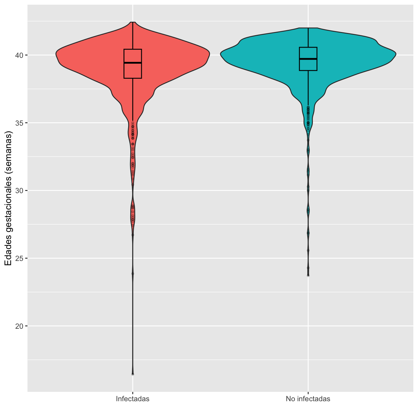
Figura 3.6:
Ajuste de las edades gestacionales de infectadas y no infectadas a distribuciones normales: test de Shapiro-Wilks, p-valores \(10^{-33}\) y \(10^{-37}\), respectivamente
Edades gestacionales medias: test t, p-valor \(2\times 10^{-7}\), IC del 95% para la diferencia de medias [-0.71, -0.33]
Desviaciones típicas: test de Fligner-Killeen, p-valor \(10^{-5}\)
Nota: Como vemos en los boxplot, hay dos casos de infectadas con edades gestacionales incompatibles con la definición de “parto” (y que además luego tienen información incompatible con esto). Son 00133-00046 y 00268-00008. Si las quitamos, las conclusiones son las mismas:
Ajuste de las edades gestacionales de infectadas y no infectadas a distribuciones normales: test de Shapiro-Wilks, p-valores \(10^{-31}\) y \(10^{-37}\), respectivamente
Edades medias: test t, p-valor \(3\times 10^{-7}\), IC del 95% para la diferencia de medias [-0.68, -0.31]
Desviaciones típicas: test de Fligner-Killeen, p-valor \(2\times 10^{-5}\)
3.2.9 Prematuridad
| Infectadas (N) | Infectadas (%) | No infectadas (N) | No infectadas (%) | RA | Extr. Inf. IC RA | Extr. Sup. IC RA | RR | Extr. Inf. IC RA | Extr. Sup. IC RR | p-valor | |
|---|---|---|---|---|---|---|---|---|---|---|---|
| Prematuro | 104 | 11.9 | 75 | 6.3 | 0.0556 | 0.0292 | 0.0821 | 1.88 | 1.42 | 2.5 | 1.18e-05 |
| No prematuro | 773 | 88.1 | 1116 | 93.7 | |||||||
| Datos perdidos | 0 | 0 |
3.2.10 Eventos trombóticos
I=Casos$EVENTOS_TROMBO_TOTALES
NI1=Controls$DVT
NI2=Controls$PE
NI=rep(NA,n_NI)
for (i in 1:n_NI){NI[i]=max(NI1[i],NI2[i],na.rm=TRUE)}
NI=factor(NI,levels=0:1)
Tabla.DMGC(I,NI,"No eventos trombóticos","Eventos trombóticos")| Infectadas (N) | Infectadas (%) | No infectadas (N) | No infectadas (%) | RA | Extr. Inf. IC RA | Extr. Sup. IC RA | RR | Extr. Inf. IC RA | Extr. Sup. IC RR | p-valor | |
|---|---|---|---|---|---|---|---|---|---|---|---|
| Eventos trombóticos | 7 | 0.8 | 0 | 0 | 0.008 | 0.0011 | 0.0149 | Inf | 2.48 | Inf | 0.0024 |
| No eventos trombóticos | 870 | 99.2 | 1191 | 100 | |||||||
| Datos perdidos | 0 | 416 |
3.2.11 Eventos hemorrágicos
I=Casos$EVENTOS_HEMORRAGICOS_TOTAL
NI=Controls$eventos_hemorragicos
Tabla.DMGC(I,NI,"No eventos heomorrágicos","Eventos hemorrágicos")| Infectadas (N) | Infectadas (%) | No infectadas (N) | No infectadas (%) | RA | Extr. Inf. IC RA | Extr. Sup. IC RA | RR | Extr. Inf. IC RA | Extr. Sup. IC RR | p-valor | |
|---|---|---|---|---|---|---|---|---|---|---|---|
| Eventos hemorrágicos | 51 | 5.8 | 64 | 5.4 | 0.0044 | -0.0167 | 0.0255 | 1.08 | 0.76 | 1.54 | 0.6981 |
| No eventos heomorrágicos | 826 | 94.2 | 1127 | 94.6 | |||||||
| Datos perdidos | 0 | 0 |
3.2.12 Ingreso materno en UCI
| Infectadas (N) | Infectadas (%) | No infectadas (N) | No infectadas (%) | RA | Extr. Inf. IC RA | Extr. Sup. IC RA | RR | Extr. Inf. IC RA | Extr. Sup. IC RR | p-valor | |
|---|---|---|---|---|---|---|---|---|---|---|---|
| UCI | 24 | 2.7 | 2 | 0.2 | 0.0257 | 0.0137 | 0.0377 | 16.3 | 4.28 | 62.14 | 1e-07 |
| No UCI | 853 | 97.3 | 1189 | 99.8 | |||||||
| Datos perdidos | 0 | 0 |
3.2.13 Ingreso materno en UCI según el momento del parto o cesárea
UCI.I=sum(Casos$UCI,na.rm=TRUE)
UCI.NI=sum(Controls$UCI...9,na.rm=TRUE)
I=Casos$UCI_ANTES.DESPUES.DEL.PARTO
NI=Controls$UCI.ANTES.DEL.PARTO  #Vacía
NA_I=length(I[is.na(I)])
NA_NI=length(NI[is.na(NI)])


EE=rbind(as.vector(table(I)),
         c(0,UCI.NI))
FT=fisher.test(EE)
PT=prop.test(EE[,1],rowSums(EE))

RA=round(PT$estimate[1]-PT$estimate[2],3)
ICRA=round(PT$conf.int,4)
RR=round(PT$estimate[1]/PT$estimate[2],2)
ICRR=round(RelRisk(EE,conf.level=0.95,method="score")[2:3],2)

EEExt=rbind(c(as.vector(table(I))[2:1],NA_I),
            c(round(100*as.vector(table(I))[2:1]/(UCI.I-NA_I),1),NA),
            c(as.vector(c(0,UCI.NI))[2:1],NA_NI),
            c(round(100*as.vector(c(0,UCI.NI))[2:1]/(UCI.NI-NA_NI),1),NA),
            c(RA,NA,NA),
            c(ICRA[1],NA,NA),
            c(ICRA[2],NA,NA),
            c(RR,NA,NA),
            c(ICRR[1],NA,NA),
            c(ICRR[2],NA,NA),
            c(round(FT$p.value,4),NA,NA)
            )

colnames(EEExt)=c("Después del parto","Antes del parto" ,"Datos perdidos")
rownames(EEExt)=c("Infectadas (N)", "Infectadas (%)","No infectadas (N)", "No infectadas (%)","RA","Extr. Inf. IC RA","Extr. Sup. IC RA","RR","Extr. Inf. IC RA","Extr. Sup. IC RR", "p-valor")


t(EEExt) %>%
  kbl() %>%
  kable_styling() %>%
scroll_box(width="100%", box_css="border: 0px;")| Infectadas (N) | Infectadas (%) | No infectadas (N) | No infectadas (%) | RA | Extr. Inf. IC RA | Extr. Sup. IC RA | RR | Extr. Inf. IC RA | Extr. Sup. IC RR | p-valor | |
|---|---|---|---|---|---|---|---|---|---|---|---|
| Después del parto | 20 | -2.4 | 2 | -0.2 | 0.167 | -0.1491 | 0.4824 | Inf | 0.18 | Inf | 1 |
| Antes del parto | 4 | -0.5 | 0 | 0.0 | |||||||
| Datos perdidos | 853 | 1191 |
3.2.14 Embarazos con algún feto muerto anteparto
I=Casos$Feto.muerto.intraútero
I[I=="Sí"]=1
I[I=="No"]=0
NI1=Controls$Feto.vivo...194
NI1[NI1=="Sí"]=0
NI1[NI1=="No"]=1
NI2=Controls$Feto.vivo...245
NI2[NI2=="Sí"]=0
NI2[NI2=="No"]=1
NI=NI1
for (i in 1:length(NI1)){NI[i]=max(NI1[i],NI2[i],na.rm=TRUE)}

Tabla.DMGC(I,NI,"Ningún feto muerto anteparto","Algún feto muerto anteparto")| Infectadas (N) | Infectadas (%) | No infectadas (N) | No infectadas (%) | RA | Extr. Inf. IC RA | Extr. Sup. IC RA | RR | Extr. Inf. IC RA | Extr. Sup. IC RR | p-valor | |
|---|---|---|---|---|---|---|---|---|---|---|---|
| Algún feto muerto anteparto | 9 | 1 | 3 | 0.3 | 0.0077 | -5e-04 | 0.016 | 4.07 | 1.2 | 13.88 | 0.0359 |
| Ningún feto muerto anteparto | 868 | 99 | 1188 | 99.7 | |||||||
| Datos perdidos | 0 | 0 |
3.2.15 Inicio del parto
I=Casos$Inicio.de.parto
I=factor(Casos$Inicio.de.parto,levels=c("Espontáneo", "Inducido", "Cesárea"),ordered=TRUE)
NI=Controls$Inicio.de.parto
NI[NI=="Cesárea programada"]="Cesárea"
NI=factor(NI,levels=c("Espontáneo", "Inducido", "Cesárea"),ordered=TRUE)

Tabla.DMGCm(I,NI,c("Espontáneo", "Inducido", "Cesárea"),r=9)| Infectadas (N) | Infectadas (%) | No infectadas (N) | No infectadas (%) | RA | Extr. Inf. IC RA | Extr. Sup. IC RA | RR | Extr. Inf. IC RA | Extr. Sup. IC RR | p-valor | |
|---|---|---|---|---|---|---|---|---|---|---|---|
| Espontáneo | 442 | 50.5 | 734 | 61.6 | -0.1111 | -0.1553 | -0.0670 | 0.820 | 0.757 | 0.887 | 0.0000018 |
| Inducido | 325 | 37.1 | 393 | 33.0 | 0.0415 | -0.0012 | 0.0841 | 1.126 | 1.000 | 1.267 | 0.1656893 |
| Cesárea | 108 | 12.3 | 64 | 5.4 | 0.0697 | 0.0434 | 0.0960 | 2.297 | 1.709 | 3.087 | 0.0000001 |
| Datos perdidos | 2 | 0 |
df =data.frame(
  Factor=c( rep("Infectadas",length(I)), rep("No infectadas",length(NI))),
  Inicios=ordered(c( I,NI ),levels=c("Espontáneo","Inducido","Cesárea"))
)

base=ordered(rep(c("Espontáneo","Inducido","Cesárea"), each=2),levels=c("Espontáneo","Inducido","Cesárea"))
Grupo=rep(c("Infectada","No infectada") , 3)
valor=c(as.vector(prop.table(table(df),margin=1))                 )
data <- data.frame(base,Grupo,valor)


ggplot(data, aes(fill=base, y=valor, x=Grupo)) +
  geom_bar(position="dodge", stat="identity")+
  ylab("")+
  scale_fill_brewer(palette = "Set3")+
  labs(fill = "Inicio de parto")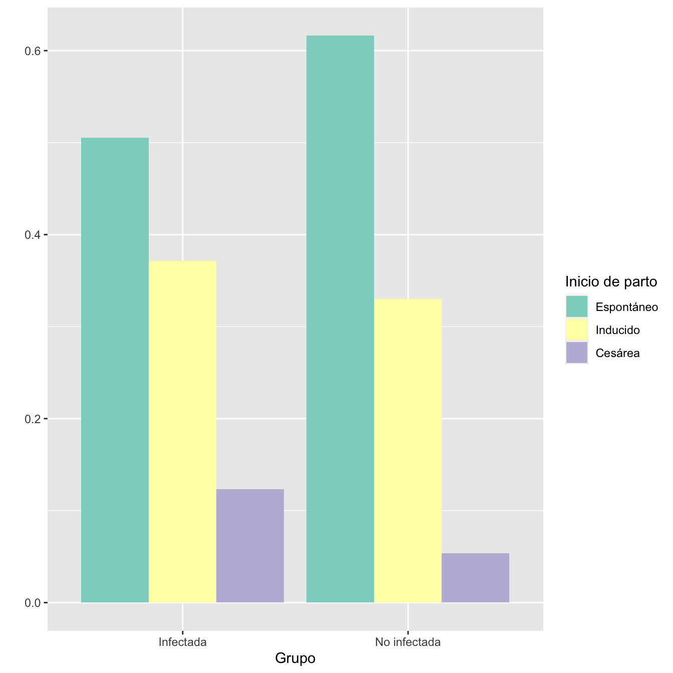
Figura 3.7:
df =data.frame(
  Factor=c( rep("Infectadas",length(I)), rep("No infectadas",length(NI))),
  Inicios=ordered(c( I,NI ),levels=c("Espontáneo","Inducido","Cesárea"))
)

base=ordered(rep(c("Espontáneo","Inducido","Cesárea"), each=2),levels=c("Espontáneo","Inducido","Cesárea"))
Grupo=rep(c("Infectada","No infectada") , 3)
valor=c(as.vector(prop.table(table(df),margin=2))                 )
data <- data.frame(base,Grupo,valor)


ggplot(data, aes(fill=Grupo, y=valor, x=base)) +
  geom_bar(position="dodge", stat="identity")+
  xlab("Inicios de parto")+
  ylab("")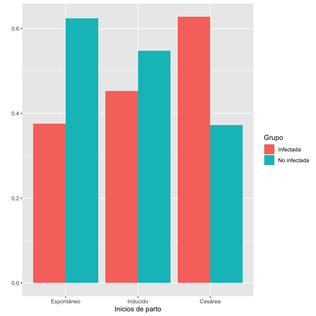
Figura 3.8:
- Distribuciones de los inicios de parto en los grupos de infectadas y no infectadas: test \(\chi^2\), p-valor \(5\times 10^{-10}\)
3.2.16 Tipo de parto
I.In=Casos$Inicio.de.parto
I.In[I.In=="Cesárea"]="Cesárea programada"
I=Casos$Tipo.de.parto
I[I.In=="Cesárea programada"]="Cesárea programada"
I[I=="Cesárea"]="Cesárea urgente"
I[I=="Eutocico"]="Eutócico"
I=factor(I,levels=c("Eutócico", "Instrumental", "Cesárea programada", "Cesárea urgente"),ordered=TRUE)

NI.In=Controls$Inicio.de.parto
NI=Controls$Tipo.de.parto
NI[NI.In=="Cesárea programada"]="Cesárea programada"
NI[NI=="Cesárea"]="Cesárea urgente"
NI[NI=="Eutocico"]="Eutócico"
NI=factor(NI,levels=c("Eutócico", "Instrumental", "Cesárea programada", "Cesárea urgente"),ordered=TRUE)

Tabla.DMGCm(I,NI,c("Eutócico", "Instrumental", "Cesárea programada", "Cesárea urgente"),r=6)| Infectadas (N) | Infectadas (%) | No infectadas (N) | No infectadas (%) | RA | Extr. Inf. IC RA | Extr. Sup. IC RA | RR | Extr. Inf. IC RA | Extr. Sup. IC RR | p-valor | |
|---|---|---|---|---|---|---|---|---|---|---|---|
| Eutócico | 528 | 60.2 | 767 | 64.4 | -0.0419 | -0.0852 | 0.0013 | 0.935 | 0.873 | 1.001 | 0.214018 |
| Instrumental | 100 | 11.4 | 177 | 14.9 | -0.0346 | -0.0647 | -0.0044 | 0.767 | 0.610 | 0.964 | 0.089513 |
| Cesárea programada | 108 | 12.3 | 64 | 5.4 | 0.0694 | 0.0432 | 0.0956 | 2.292 | 1.705 | 3.080 | 0.000000 |
| Cesárea urgente | 141 | 16.1 | 183 | 15.4 | 0.0071 | -0.0257 | 0.0399 | 1.046 | 0.856 | 1.280 | 1.000000 |
| Datos perdidos | 0 | 0 |
df =data.frame(
  Factor=c( rep("Infectadas",length(I)), rep("No infectadas",length(NI))),
  Inicios=ordered(c( I,NI ),levels=c("Eutócico", "Instrumental", "Cesárea programada", "Cesárea urgente"))
)

base=ordered(rep(c("Eutócico", "Instrumental", "Cesárea prog.", "Cesárea urg."), each=2),levels=c("Eutócico", "Instrumental", "Cesárea prog.", "Cesárea urg."))
Grupo=rep(c("Infectada","No infectada") , 4)
valor=c(as.vector(prop.table(table(df),margin=1))                 )
data <- data.frame(base,Grupo,valor)


ggplot(data, aes(fill=base, y=valor, x=Grupo)) +
  geom_bar(position="dodge", stat="identity")+
  ylab("")+
  scale_fill_brewer(palette = "Set3")+
  labs(fill = "Tipo de parto")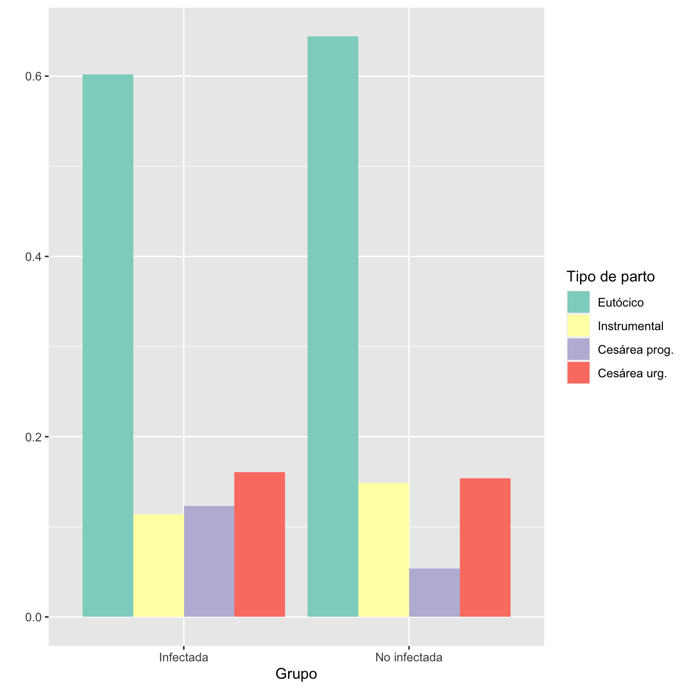
Figura 3.9:
df =data.frame(
  Factor=c( rep("Infectadas",length(I)), rep("No infectadas",length(NI))),
  Inicios=ordered(c( I,NI ),levels=c("Eutócico", "Instrumental", "Cesárea programada", "Cesárea urgente"))
)

base=ordered(rep(c("Eutócico", "Instrumental", "Cesárea prog.", "Cesárea urg."), each=2),levels=c("Eutócico", "Instrumental", "Cesárea prog.", "Cesárea urg."))
Grupo=rep(c("Infectada","No infectada") , 4)
valor=as.vector(prop.table(table(df), margin=2))
data <- data.frame(base,Grupo,valor)


ggplot(data, aes(fill=Grupo, y=valor, x=base)) +
  geom_bar(position="dodge", stat="identity")+
  xlab("Tipos de parto")+
  ylab("")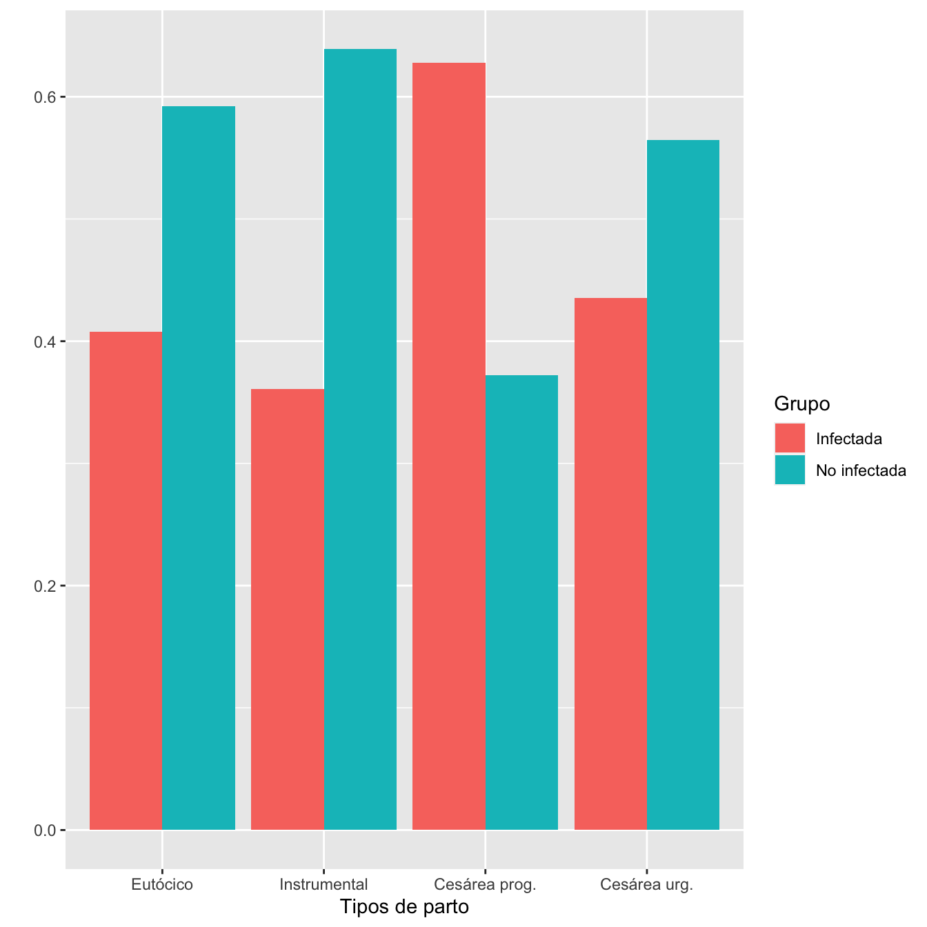
Figura 3.10:
- Distribuciones de los tipos de parto en los grupos de infectadas y no infectadas: test \(\chi^2\), p-valor \(10^{-7}\)
3.2.17 Hemorragias postparto
I=Casos$Hemorragia.postparto
I.sino=I
I.sino[!is.na(I.sino)& I.sino!="No"]="Sí"
I=ordered(I,levels=names(table(I))[c(2,3,1,4)])


NI=Controls$Hemorragia.postparto
NI.sino=NI
NI.sino[!is.na(NI.sino)& NI.sino!="No"]="Sí"
NI=ordered(NI,levels=names(table(NI))[c(2,3,1,4)])

Tabla.DMGC(I.sino,NI.sino,"No HPP","HPP")| Infectadas (N) | Infectadas (%) | No infectadas (N) | No infectadas (%) | RA | Extr. Inf. IC RA | Extr. Sup. IC RA | RR | Extr. Inf. IC RA | Extr. Sup. IC RR | p-valor | |
|---|---|---|---|---|---|---|---|---|---|---|---|
| HPP | 41 | 4.8 | 50 | 4.3 | 0.0053 | -0.0142 | 0.0247 | 1.12 | 0.75 | 1.68 | 0.5884 |
| No HPP | 814 | 95.2 | 1121 | 95.7 | |||||||
| Datos perdidos | 22 | 20 |
Tabla.DMGCm(I,NI,c("HPP tratamiento médico" ,
"HPP tratamiento quirúrgico conservador",
"Histerectomía obstétrica"    ,
"No") ,r=6)| Infectadas (N) | Infectadas (%) | No infectadas (N) | No infectadas (%) | RA | Extr. Inf. IC RA | Extr. Sup. IC RA | RR | Extr. Inf. IC RA | Extr. Sup. IC RR | p-valor | |
|---|---|---|---|---|---|---|---|---|---|---|---|
| HPP tratamiento médico | 32 | 3.7 | 42 | 3.6 | 0.0016 | -0.0160 | 0.0192 | 1.043 | 0.667 | 1.633 | 1.000000 |
| HPP tratamiento quirúrgico conservador | 4 | 0.5 | 7 | 0.6 | -0.0013 | -0.0087 | 0.0061 | 0.783 | 0.244 | 2.510 | 1.000000 |
| Histerectomía obstétrica | 5 | 0.6 | 1 | 0.1 | 0.0050 | -0.0014 | 0.0114 | 6.848 | 1.128 | 41.562 | 0.355572 |
| No | 814 | 95.2 | 1121 | 95.7 | -0.0053 | -0.0247 | 0.0142 | 0.995 | 0.976 | 1.014 | 1.000000 |
| Datos perdidos | 22 | 20 |
df =data.frame(
  Factor=c( rep("Infectadas",length(I[I!="No"])), rep("No infectadas",length(NI[NI!="No"]))),
  Hemos=ordered(c( I[I!="No"],NI[NI!="No"] ),levels=names(table(I))[-4])
)

base=ordered(rep(c("Tto. médico", "Tto. Qx conservador", "Histerectomía"), each=2),levels=c("Tto. médico", "Tto. Qx conservador", "Histerectomía"))
Grupo=rep(c("Infectada","No infectada") , 3)
valor=as.vector(prop.table(table(df), margin=1))
data <- data.frame(base,Grupo,valor)


ggplot(data, aes(fill=Grupo, y=valor, x=base)) +
  geom_bar(position="dodge", stat="identity")+
  xlab("Tratamientos de hemorragia postparto")+
  ylab("")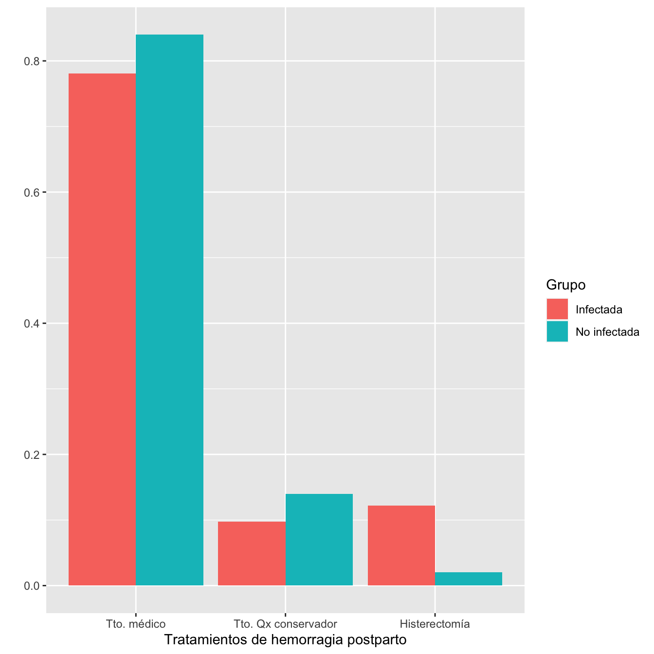
Figura 3.11:
Distribuciones de los tipos de hemorragia postparto (incluyendo Noes) en los grupos de infectadas y no infectadas: test \(\chi^2\) de Montercarlo, p-valor 0.24
Distribuciones de los tipos de hemorragia postparto en los grupos de infectadas y no infectadas que tuvieron hemorragia postparto: test \(\chi^2\) de Montercarlo, p-valor 1
3.2.18 Fetos muertos anteparto
I1=Casos$Feto.muerto.intraútero
I1[I1=="Sí"]="Muerto"
I1[I1=="No"]="Vivo"
I2=CasosGM$Feto.vivo
I2[I2=="Sí"]="Vivo"
I2[I2=="No"]="Muerto"
I=c(I1,I2)
I=ordered(I,levels=c("Vivo","Muerto"))


n_IFT=length(I)
n_VI=as.vector(table(I))[1]NI1=Controls$Feto.vivo...194
NI2=ControlsGM$Feto.vivo...245
NI=c(NI1,NI2)
NI[NI=="Sí"]="Vivo"
NI[NI=="No"]="Muerto"
NI=ordered(NI,levels=c("Vivo","Muerto"))
n_NIFT=length(NI)
n_VNI=as.vector(table(NI))[1]
Tabla.DMGC(I,NI,"Feto vivo","Feto muerto anteparto")| Infectadas (N) | Infectadas (%) | No infectadas (N) | No infectadas (%) | RA | Extr. Inf. IC RA | Extr. Sup. IC RA | RR | Extr. Inf. IC RA | Extr. Sup. IC RR | p-valor | |
|---|---|---|---|---|---|---|---|---|---|---|---|
| Feto muerto anteparto | 9 | 1 | 3 | 0.2 | 0.0076 | -5e-04 | 0.0157 | 4.08 | 1.2 | 13.92 | 0.0358 |
| Feto vivo | 885 | 99 | 1214 | 99.8 | |||||||
| Datos perdidos | 1 | 2 |
3.2.19 Peso de neonatos al nacimiento
I=c(Casos[Casos$Feto.muerto.intraútero=="No",]$Peso._gramos_...125,CasosGM[CasosGM$Feto.vivo=="Sí",]$Peso._gramos_...148)
NI=c(Controls[Controls$Feto.vivo...194=="Sí",]$Peso._gramos_...198,ControlsGM[ControlsGM$Feto.vivo...245=="Sí",]$Peso._gramos_...247)
data =data.frame(
name=c(rep("Hijos de infectadas",length(I)), rep("Hijos de no infectadas",length(NI))),
Pesos=c(I,NI)
)
sample_size = data %>% group_by(name) %>% summarize(num=n())
data %>%
left_join(sample_size) %>%
mutate(myaxis = paste0(name, "\n", "n=", num)) %>%
ggplot( aes(x=myaxis, y=Pesos, fill=name)) +
geom_violin(width=0.9) +
geom_boxplot(width=0.1, color="black", alpha=0.2,outlier.fill="black",
outlier.size=1) +
theme(
legend.position="none",
plot.title = element_text(size=11)
) +
xlab("")+
ylab("Pesos (gramos)")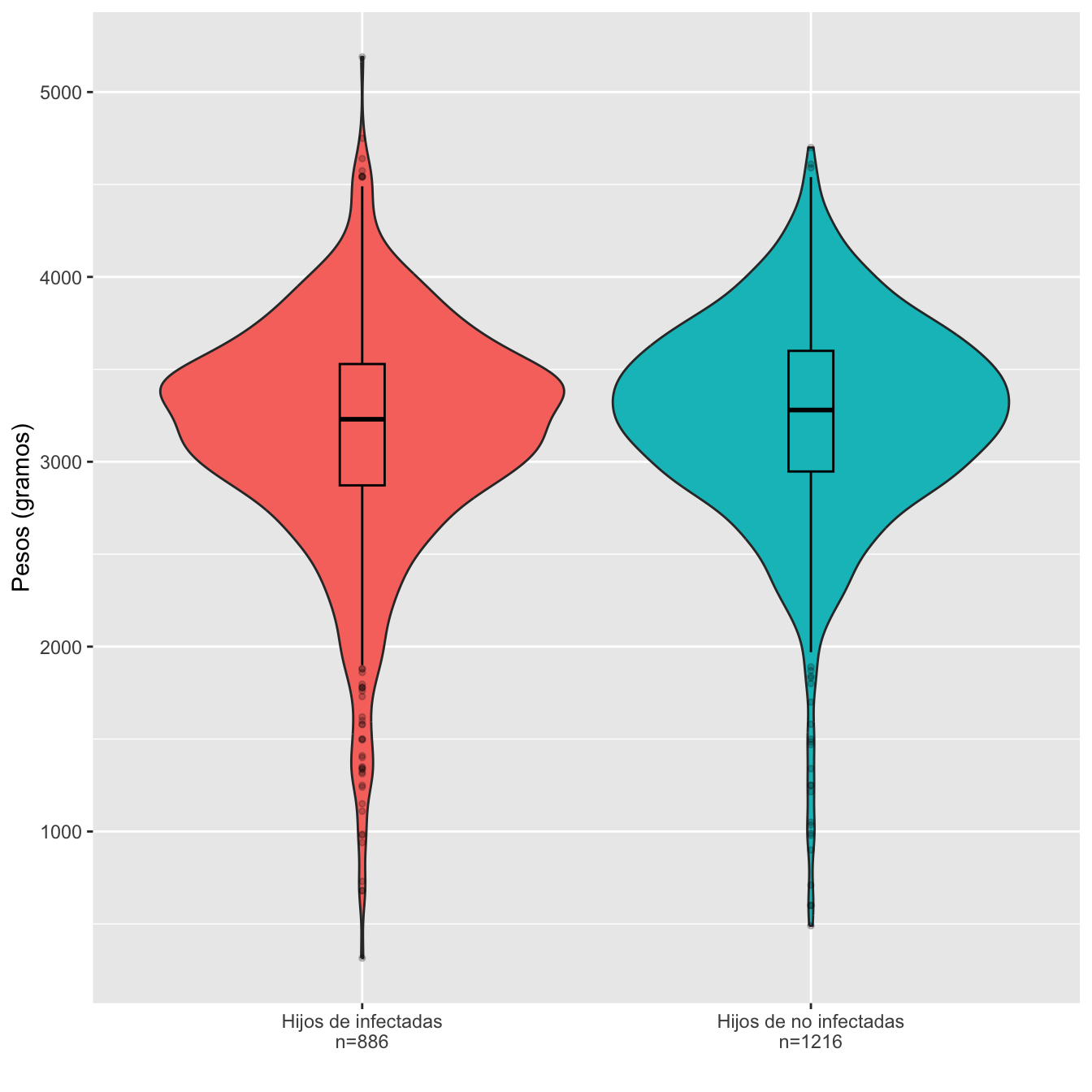
Figura 3.12:
Dades=rbind(c(min(I,na.rm=TRUE),max(I,na.rm=TRUE), round(mean(I,na.rm=TRUE),1),round(median(I,na.rm=TRUE),1),round(quantile(I,c(0.25,0.75),na.rm=TRUE),1), round(sd(I,na.rm=TRUE),1)),
            c(min(NI,na.rm=TRUE),max(NI,na.rm=TRUE), round(mean(NI,na.rm=TRUE),1),round(median(NI,na.rm=TRUE),1),round(quantile(NI,c(0.25,0.75),na.rm=TRUE),1),round(sd(NI,na.rm=TRUE),1)))

colnames(Dades)=c("Peso mínimo","Peso máximo","Peso medio", "Peso mediano", "1er cuartil", "3er cuartil", "Desv. típica")
rownames(Dades)=c("Infectadas", "No infectadas")

Dades %>%
  kbl() %>%
  kable_styling() %>%
scroll_box(width="100%", box_css="border: 0px;")| Peso mínimo | Peso máximo | Peso medio | Peso mediano | 1er cuartil | 3er cuartil | Desv. típica | |
|---|---|---|---|---|---|---|---|
| Infectadas | 315 | 5190 | 3157.3 | 3230 | 2872.5 | 3528.8 | 615.8 |
| No infectadas | 490 | 4700 | 3242.9 | 3280 | 2947.5 | 3600.0 | 549.6 |
Ajuste de los pesos de hijos de infectadas y no infectadas a distribuciones normales: test de Shapiro-Wilks, p-valores \(2\times 10^{-16}\) y \(6\times 10^{-18}\), respectivamente
Pesos medios: test t, p-valor 0.0011, IC del 95% para la diferencia de medias [-136.93, -34.13]
Desviaciones típicas: test de Fligner-Killeen, p-valor 0.0811
Definimos bajo peso a peso menor o igual a 2500 g. Un 9.21% del total de neonatos no muesrtos anteparto son de bajo peso con esta definición.
I.cut=cut(I,breaks=c(0,2500,10000),labels=c(1,0),right=FALSE)
I.cut=ordered(I.cut,levels=c(0,1))
NI.cut=cut(NI,breaks=c(0,2500,10000),labels=c(1,0),right=FALSE)
NI.cut=ordered(NI.cut,levels=c(0,1))

Tabla.DMGC(I.cut,NI.cut,"No bajo peso","Bajo peso")| Infectadas (N) | Infectadas (%) | No infectadas (N) | No infectadas (%) | RA | Extr. Inf. IC RA | Extr. Sup. IC RA | RR | Extr. Inf. IC RA | Extr. Sup. IC RR | p-valor | |
|---|---|---|---|---|---|---|---|---|---|---|---|
| Bajo peso | 100 | 11.5 | 91 | 7.6 | 0.0394 | 0.0124 | 0.0663 | 1.52 | 1.16 | 1.99 | 0.0026 |
| No bajo peso | 770 | 88.5 | 1113 | 92.4 | |||||||
| Datos perdidos | 16 | 12 |
3.2.20 Apgar
I=c(Casos$APGAR.5...126,CasosGM$APGAR.5...150)
I[I==19]=NA
NI=c(Controls$APGAR.5...200,ControlsGM$APGAR.5...249)

I.5=cut(I,breaks=c(-1,7,20),labels=c("0-7","8-10"))
NI.5=cut(NI,breaks=c(-1,7,20),labels=c("0-7","8-10"))
I.5=ordered(I.5,levels=c("8-10","0-7"))
NI.5=ordered(NI.5,levels=c("8-10","0-7"))

Tabla.DMGC(I.5,NI.5,"Apgar.5≥8","Apgar.5≤7")| Infectadas (N) | Infectadas (%) | No infectadas (N) | No infectadas (%) | RA | Extr. Inf. IC RA | Extr. Sup. IC RA | RR | Extr. Inf. IC RA | Extr. Sup. IC RR | p-valor | |
|---|---|---|---|---|---|---|---|---|---|---|---|
| Apgar.5≤7 | 26 | 2.9 | 28 | 2.3 | 0.0062 | -0.0087 | 0.0212 | 1.27 | 0.75 | 2.14 | 0.4038 |
| Apgar.5≥8 | 860 | 97.1 | 1183 | 97.7 | |||||||
| Datos perdidos | 9 | 8 |
3.2.21 Ingreso de neonatos vivos en UCIN
I=c(Casos[Casos$Feto.muerto.intraútero=="No",]$Ingreso.en.UCIN,CasosGM[CasosGM$Feto.vivo=="Sí",]$Ingreso.en.UCI)
NI=c(Controls[Controls$Feto.vivo...194=="Sí",]$Ingreso.en.UCI...213,ControlsGM[ControlsGM$Feto.vivo...245=="Sí",]$Ingreso.en.UCI...260)

Tabla.DMGC(I,NI,"No UCIN","UCIN")| Infectadas (N) | Infectadas (%) | No infectadas (N) | No infectadas (%) | RA | Extr. Inf. IC RA | Extr. Sup. IC RA | RR | Extr. Inf. IC RA | Extr. Sup. IC RR | p-valor | |
|---|---|---|---|---|---|---|---|---|---|---|---|
| UCIN | 93 | 10.6 | 34 | 2.8 | 0.0779 | 0.0545 | 0.1013 | 3.76 | 2.57 | 5.51 | 0 |
| No UCIN | 784 | 89.4 | 1173 | 97.2 | |||||||
| Datos perdidos | 9 | 9 |